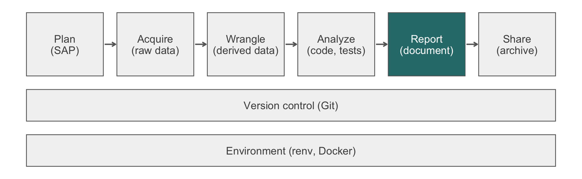
32 Ethics Beyond Compliance
In 2016 two researchers scraped some 70,000 profiles from the dating site OkCupid and posted them to an open research repository: usernames beside answers to intimate questions about sexuality, drug use, and politics. Asked about consent, they replied that the data were already public. That was true, but it did not answer the question (Zimmer, 2016). Every user had disclosed each answer to an audience of their choosing. The release joined the disclosures into one permanent, searchable file attached to the names people use. No number in it was false, and no regulation the researchers recognized stopped them. This chapter is about failures of that kind, in which every rule is followed and readers or participants are still misled or harmed. It is also about why the statistician, not the institutional review board (IRB), is often the last person who can stop them.
The first principle is that you must not fool yourself, and you are the easiest person to fool.
Richard P. Feynman, Cargo Cult Science (1974)
NoteIn this chapter
Reading time. About 30 minutes.
You’ll need. Chapter 4 for quasi-identifiers, Chapter 3 for the registers of a claim, and Chapter 20 for ggplot2. The code uses:
You’ll be able to.
- Name, for each of five recurring failures, where in the workflow it enters and what catches it.
- Distinguish research misconduct (fabrication, falsification, plagiarism) from questionable research practices, and name the professional standard each violates.
- Rewrite causal language attached to associational evidence, and state the causal question and its assumptions explicitly when the question is causal.
- Demonstrate why overlapping confidence intervals do not imply a non-significant difference, and state the groups to which an estimate does and does not transport.
Outline.
NoteSkip ahead?
If these answers come quickly, skip to the next chapter. The answers are in Section 32.12.
- A dataset is assembled entirely from information that individuals published about themselves in public. Explain how releasing it can nonetheless harm them.
- Two group means have 95% confidence intervals that overlap. May you conclude that the groups do not differ significantly?
- Name three ways a figure can mislead a reader without containing a single false number.
32.1 Compliance is a floor
The regulatory chapters of this book describe a floor. Chapter 34 covers what the funders require, Chapter 4 what the Health Insurance Portability and Accountability Act (HIPAA) Privacy Rule requires, and Chapter 28 what the Food and Drug Administration requires. Clearing that floor is necessary for defensible practice and nowhere near sufficient. The floor is written in terms of procedures, and the failures that matter most are failures of inference.
32.1.1 Five failures and where each is caught
Five such failures recur in biomedical work, and they share a structure: at no point does anyone state a falsehood. The data are real, and the computation is correct. The p-value is what the software returned, and the figure plots the numbers it claims to plot. The reader is misled in the gap between what was computed and what the reader concludes. Table 32.1 is the map for the rest of the chapter. Each failure enters the workflow at a different point, so each is caught at a different point.
| Failure | Introduced at | Caught by |
|---|---|---|
| Aggregation harm | Data acquisition and scraping (Chapter 14) | Asking, before you assemble, whether the people in the data would be surprised |
| Causal overclaiming | The Results-to-Discussion transition | Reading your own discussion for causal verbs; peer review (Chapter 33) |
| Visual misrepresentation | Figure construction (Chapter 20) | Asking what the reader’s eye is measuring |
| Overlapping-interval fallacy | Interpretation, and often the figure | Reporting the contrast, not the arms |
| Unrepresentative sample | Study design and recruitment; sometimes acquisition | Reporting who was sampled beside who the result is for; a proxy audit before a model acts |
The infrastructure of this book does not address whether an analysis misleads. Reproducibility guarantees only that a wrong conclusion can be regenerated exactly.
32.1.2 You are the last person who can catch it
The clinical collaborator cannot evaluate whether the confidence interval supports the sentence in the abstract. That is why they have you. The reviewer may or may not look, and the reader certainly will not. Suppose the press release says ‘exercise prevents cancer’, and your analysis found an association in an observational cohort of volunteers. You are then the last chance to correct that sentence.
Distortion is usually accidental, which does not make it harmless. Almost nobody sets out to deceive with a truncated axis. They set out to make the effect visible, and a truncated axis makes it visible. The standard is what a competent reader would conclude, whatever the intent.
NoteCheck
Question. A paper reports an observational study. The IRB approved it, the data are de-identified under Safe Harbor, the Data Management and Sharing Plan (DMSP) is in place, the code is on Zenodo with a digital object identifier (DOI), and every number is correctly computed. The abstract concludes that the intervention ‘reduces 30-day readmission’. Has anything gone wrong?
Answer. Yes, and nothing in the compliance apparatus was built to catch it. What is wrong is a verb. An observational design licenses ‘was associated with lower readmission’, not ‘reduces’. A guideline committee or a health system deciding where to spend money will act on ‘reduces’, and the evidence does not support the action. Reproducibility, compliance, and correct computation are each necessary, but together they are not sufficient. Only the analyst can close the gap.
32.2 Professional standards and misconduct
The profession has written its obligations down. The American Statistical Association’s Ethical Guidelines for Statistical Practice, approved by its Board in February 2022 (American Statistical Association, 2022), apply to anyone who practices statistics, whatever their title. They are organized as eight principles, and most of this book’s habits are instances of one of them (Table 32.2).
| ASA principle | What it asks of you | Where this book practices it |
|---|---|---|
| A. Professional integrity and accountability | Methods you can defend; honesty about limitations | Every Verification callout |
| B. Integrity of data and methods | Report data and methods so others can assess them; disclose what you removed | Chapter 26, Chapter 21 |
| C. Responsibilities to stakeholders | Clear statements of what the results support | Chapter 33 |
| D. Responsibilities to research subjects and data subjects | Protect privacy and confidentiality; consider harms | Chapter 4; aggregation harm, below |
| E. Responsibilities to members of multidisciplinary teams | Respect others’ expertise; make your own explicit | Chapter 3 |
| F. Responsibilities to fellow practitioners and the profession | Share methods; review fairly | Section 33.9 |
| G. Responsibilities of leaders, supervisors, and mentors | Foster an environment where these can be followed | Code review, Chapter 8 |
| H. Responsibilities regarding potential misconduct | Avoid condoning it; report it through proper channels | This section |
32.2.1 Misconduct and questionable practices
Research misconduct has a federal definition: fabrication, falsification, or plagiarism in proposing, performing, or reviewing research, or in reporting its results (Office of Science and Technology Policy, 2000). Fabrication is making up data or results. Falsification is manipulating materials, processes, or data, or changing or omitting data or results, so that the research record misrepresents the research. Plagiarism is taking another’s ideas, processes, results, or words without credit. Honest error and differences of opinion are excluded. For a statistician, the clause to remember is ‘omitting data or results’. Dropping the patients who spoil an estimate, without disclosure, is falsification, however it is labeled in the code.
Between misconduct and good practice lies a wider band of questionable research practices (QRPs). Surveys of researchers find them to be common (John et al., 2012). They are rarely fraud, but they frequently decide the result:
| Practice | What it looks like | What prevents it |
|---|---|---|
| HARKing (hypothesizing after the results are known) | A hypothesis formed from the data presented as if stated in advance (Kerr, 1998) | A tagged analysis plan (Chapter 26) |
| Undisclosed analytic flexibility | Trying exclusions, covariates, or outcomes until one is significant (Simmons et al., 2011) | Pre-specification; reporting every analysis run |
| Selective reporting | Publishing the outcomes or subgroups that worked | Registration; reporting against the plan |
| Optional stopping | Adding patients until p crosses 0.05 | A pre-specified sample size or stopping rule |
| Unreported exclusions | Dropping ‘outliers’ without a stated rule | A rule written before the data; a flow diagram |
32.2.2 Refusing is part of the job
There is a point at which the correct professional act is to decline. That may mean refusing to sign the manuscript, refusing to produce the figure as specified, or saying that you will not perform the analysis as requested. Chapter 3 distinguishes preference from principle so that you spend your credibility on the cases where it matters. Table 32.3 and the five failures of this chapter are the catalog of those cases. Principle H of the ASA guidelines adds a harder obligation. When you suspect misconduct by someone else, raise it through your institution’s research integrity office. Do not ignore it, and do not accuse anyone in public.
32.2.3 Exercises
- Classify each as research misconduct, a questionable research practice, or acceptable, and say why: (a) an analyst removes 12 patients whose outcomes ‘looked wrong’ and reports the remaining count as the sample; (b) a paper’s introduction presents a subgroup hypothesis that the team formed after seeing the results; (c) an exploratory subgroup analysis is reported in the supplement and labeled exploratory; (d) a methods section copies two paragraphs from another group’s paper without attribution.
NoteSolution
- Falsification, if the removal is undisclosed: omitting data so that the record misrepresents the research. Disclosed, with a rule stated before the data, it would be an exclusion open to review. The difference is the disclosure. (b) HARKing, a QRP. The hypothesis is presented as a priori when it was not, so the reported p-value has no stated error rate. (c) Acceptable. The analysis is reported and labeled for what it is (Section 33.8). (d) Plagiarism, which the federal definition names alongside fabrication and falsification. The fact that the copied text describes a method rather than a result does not change this.
NoteCheck
Question. Why does Table 32.3 say each practice ‘turns a nominal error rate into an unknown one’, rather than ‘a false result’?
Answer. Because each practice can produce a true result. What it destroys is the ability to say how often the procedure would produce a false one. A p-value from the fifth analysis tried is not a 5% test, and nobody, including the analyst, can say what test it is. The harm is to the evidence. That is why the remedy is a plan dated before the data.
32.3 Aggregation harm
The OkCupid release is an instance of aggregation harm. It is the same phenomenon that Chapter 4 treats formally as quasi-identifiers, seen from the other direction. There, no single ordinary variable identifies anyone, but their conjunction can. Here, no single disclosure harms anyone, but their conjunction can. Both are questions about joint distributions. What makes the second an ethical question is context. Information carries an implicit expectation about where it will travel. Moving it somewhere else has consequences, even when every datum was freely given. Public is not the same as consented, and available is not the same as ethical. That is, the question ‘may I’ has a legal answer and an ethical one. Ask what happens to a person in your data if the analysis is right, and then what happens if it is wrong.
Before you assemble a dataset from public sources, ask the three questions in Table 32.4.
| Question | Why it works | Example |
|---|---|---|
| Would the people in it be surprised? | Not ‘would they object’, which invites you to answer for them; surprise signals a violated contextual expectation | Users of a dating site finding their answers in a research repository |
| Does the aggregate reveal what the parts did not? | The harm is in the join, not the fields | A support-forum post linked to an employer name discloses a condition to the employer |
| Can it be de-identified without destroying the analysis? | If yes, do that (Chapter 4); if no, the identifiers are load-bearing and you should be able to say why | Usernames kept ‘for linkage’ that the analysis never uses |
ImportantLLM prompt
Context. I am considering releasing, for research, a dataset assembled from public profiles on a website: usernames, ages, locations, and answers to the site’s questions. I describe the fields and the site’s terms of use below; I attach no data.
Constraints. Do not answer from legality alone. For each field and for the combination, say who the original audience was and who the release’s audience would be.
Criteria. Answer the three questions of a table like Table 32.4 for this dataset, name the harm a person in it could suffer, and say what, if anything, would make a release defensible.
Failure mode. This is the question the model is most likely to get wrong. It reasons from legality, because legality is what is written down, and it concludes that public data may be republished. It also tends to agree, and here an agreeable collaborator is worse than none. The relevant considerations exist in its training data, but it will not volunteer them unless the prompt requires them. Check. Take the question to your IRB and to a colleague who will tell you no (Section 12.3).
NoteCheck
Question. A colleague assembles a dataset entirely from public sources: forum posts, a professional registry, and voter rolls. They argue that no ethical review is needed because they disclosed nothing new. Where does the argument fail?
Answer. It treats disclosure as a property of each field rather than of the combination, and the harm is in the combination. Each source has an implicit audience, and the people in it chose exposure to that audience. Joining them creates a fact that existed nowhere before: this named person, at this address, has this condition. The keys that make the join possible are exactly the quasi-identifiers of Chapter 4. ‘Public’ also describes access, not permission. Readable data still carry terms of use, and scraping is a distinct act from reading. Finally, if assembly needs no review because each piece was public, then no aggregation ever needs review. Nobody defends that position when it is stated plainly.
32.4 Causal overclaiming
The second failure is the most common in biomedical publishing, and it usually happens in the last paragraph. An observational cohort of self-selected volunteers reports that those who exercised more had lower cancer incidence, adjusting for age, sex, smoking, and body-mass index. The finding is an association. The discussion says it ‘suggests that exercise reduces cancer risk’; the press office says exercise prevents cancer; the newspaper says it cures it. At no step did anyone fabricate a number.
The statistician’s job is to insist that the verb match the design (Habit 11). The three registers of Chapter 3 become a hierarchy of claims:
| Design | What you may say |
|---|---|
| Randomized, adequately powered, pre-specified | ’X reduced Y by \(\delta\)’ |
| Observational, well adjusted, no unmeasured confounding assumed | ‘X was associated with lower Y; the association is consistent with a causal effect but the design cannot establish one’ |
| Observational, self-selected sample, self-reported exposure | ‘Among volunteers who reported X, Y was lower. Volunteers who exercise differ from those who do not in ways we did not measure.’ |
The third row is the one to keep in view. People who exercise and report it differ systematically from people who do not. They differ along dimensions that no covariate list captures: conscientiousness, health-seeking behavior, unmeasured comorbidity, and the early symptoms of undiagnosed disease. The adjustment cannot fix this. Stating that you adjusted for age and smoking implies to a reader that it did.
The transition from Results to Discussion is where the verb changes from ‘was associated with’ to ‘reduces’ without anyone noticing. Read your own discussion as a hostile reviewer would, and search it for causal verbs. The search is mechanical enough to run as code.
causal_verbs <- c("reduc", "prevent", "protect", "caus", "lead",
"improv", "lower", "increas", "effect")
flag_causal <- function(text) {
sentences <- unlist(strsplit(text, "(?<=\\.)\\s+", perl = TRUE))
pattern <- paste0("\\b(", paste(causal_verbs, collapse = "|"),
")[a-z]*")
hits <- grepl(pattern, sentences, ignore.case = TRUE)
data.frame(flagged = hits, sentence = sentences)
}
discussion <- paste(
"Participants who exercised more had a lower incidence of cancer.",
"This suggests that regular exercise reduces cancer risk.",
"Physical activity may therefore protect against several cancers.",
"The cohort was recruited from volunteers."
)
flag_causal(discussion)
#> flagged sentence
#> 1 TRUE Participants who exercised more had a lower incidence of cancer.
#> 2 TRUE This suggests that regular exercise reduces cancer risk.
#> 3 TRUE Physical activity may therefore protect against several cancers.
#> 4 FALSE The cohort was recruited from volunteers.The first flagged sentence is an association written with a comparative (‘lower’), which is fine. The second and third are causal claims the design does not license. The search finds candidates, and you decide. That division of labor is the right one for a model too.
ImportantLLM prompt
Context. Below is the discussion section of an observational cohort study, and one sentence describing its design (volunteer cohort, self-reported exposure, adjusted for age, sex, smoking, and body-mass index).
Constraints. List every sentence whose verb implies causation. Do not rewrite the section; do not judge whether the causal claim is true.
Criteria. For each sentence, quote it, name the verb, name the design that would license it, and propose a rewrite in the register of Table 32.5 that the actual design licenses.
Failure mode. This works well, because it is a classification task rather than a judgment. Expect a few false positives, and an occasional miss where causation hides in a noun (‘the protective effect of exercise’). Check. Run flag_causal() on the same text and reconcile the two lists. Then check each flagged sentence against Table 32.5 yourself.
32.4.1 Causal foundations
None of this means causal questions are off-limits for observational data. Hernán argues that the euphemism is the problem (Hernán, 2018). Researchers who want a causal answer but write ‘associated with’ have not avoided causal inference. They have only hidden its assumptions from the reader. The remedy is to state the causal question and the assumptions under which the analysis answers it. Habit 11 and this argument agree once the question and the verb are separated. Ask the causal question openly, and let the verb in the conclusion match what the design and its stated assumptions support. Two tools make the assumptions explicit.
A directed acyclic graph (DAG) draws the assumed causal structure. Nodes are variables, and arrows are direct causal effects. The adjustment set a design needs can be read off the graph (Greenland et al., 1999). Figure 32.2 draws the exercise example. Adjusting for age and smoking closes two backdoor paths. The path through health-seeking behavior, which no one measured, stays open. That is the third row of Table 32.5 in a picture.
flowchart LR A["Age<br/><i>adjusted</i>"] --> E["Exercise"] S["Smoking<br/><i>adjusted</i>"] --> E H["Health-seeking behavior<br/><i>unmeasured</i>"] --> E E --> C["Cancer"] A --> C S --> C H --> C
Target-trial emulation asks what randomized trial you would run if you could. It then designs the observational analysis to emulate that trial, component by component: eligibility criteria, treatment strategies, assignment, the start and end of follow-up, the outcome, the causal contrast, and the analysis plan (Hernán & Robins, 2016). Its most practical benefit is the alignment of time zero. Eligibility, assignment, and the start of follow-up must coincide, as they do at randomization. Consider the immortal-time trap of the HF-HOME intake (Chapter 3), in which a patient readmitted on day 3 is counted as unvisited. It is a failure of exactly that alignment. Writing down the target trial exposes it before any code runs.
32.4.2 Exercises
- Rewrite this paragraph from a retrospective cohort study so that every verb matches the design, keeping every fact: ‘Patients who received home-health visits within a week of discharge had a 30-day readmission rate of 18%, compared with 26% among those who did not (adjusted odds ratio 0.68). Home-health visits therefore prevent readmissions, and expanding the program would reduce readmissions by a third.’
NoteSolution
‘Patients who received a home-health visit within a week of discharge had a lower 30-day readmission rate than those who did not (18% versus 26%; adjusted odds ratio 0.68). Because patients readmitted before a visit could occur are counted as unvisited, and because visited patients may differ in ways we did not measure, this comparison cannot establish whether the visits reduce readmission; a randomized comparison, or an emulated trial that aligns time zero, would be needed to estimate the effect of expanding the program.’
There are three changes. ‘Prevent’ becomes ‘had a lower rate’, the register the design licenses. The projection (‘would reduce by a third’) is removed, because it converts an association into the effect of an intervention that was never compared. Finally, the reason the design falls short is named, including the immortal-time bias specific to this comparison (Chapter 3). That is more useful to a reader than a generic ‘causation cannot be inferred’. Run flag_causal() on your rewrite. What it still flags (‘lower’, ‘reduce’) should appear only in comparative or explicitly conditional sentences.
NoteCheck
Question. A colleague cites Hernán’s argument to justify writing ‘exercise reduces cancer risk’ in the conclusion of the volunteer cohort. What is the error?
Answer. The argument licenses stating the causal question and its assumptions, not dropping the assumptions from the conclusion. Here the assumption that matters (no unmeasured confounding by health-seeking behavior) is implausible and untested. The honest conclusion is therefore the causal question, the estimate under the stated assumptions, and the reason those assumptions may fail. A causal verb with the assumptions removed is the overclaim the argument was meant to expose.
32.5 Visual misrepresentation
The third failure involves no wrong numbers, only the way they are encoded. Figure 32.3 plots the same two group means twice.
library(tidyverse)
library(patchwork)
d <- tibble(
arm = c("Control", "Treatment"),
mean = c(72.4, 74.1)
)
base <- ggplot(d, aes(arm, mean, fill = arm)) +
geom_col(width = 0.6, show.legend = FALSE) +
scale_fill_manual(values = c(Control = "#9d2235",
Treatment = "#1f4e79")) +
labs(x = NULL, y = "Score") +
theme_minimal()
p_honest <- base +
coord_cartesian(ylim = c(0, 100)) +
labs(title = "A. Axis from zero")
axis_floor <- 71
p_truncated <- base +
coord_cartesian(ylim = c(axis_floor, 75)) +
labs(title = paste("B. Axis from", axis_floor))
bar_ratio <- (d$mean[2] - axis_floor) / (d$mean[1] - axis_floor)
p_honest + p_truncated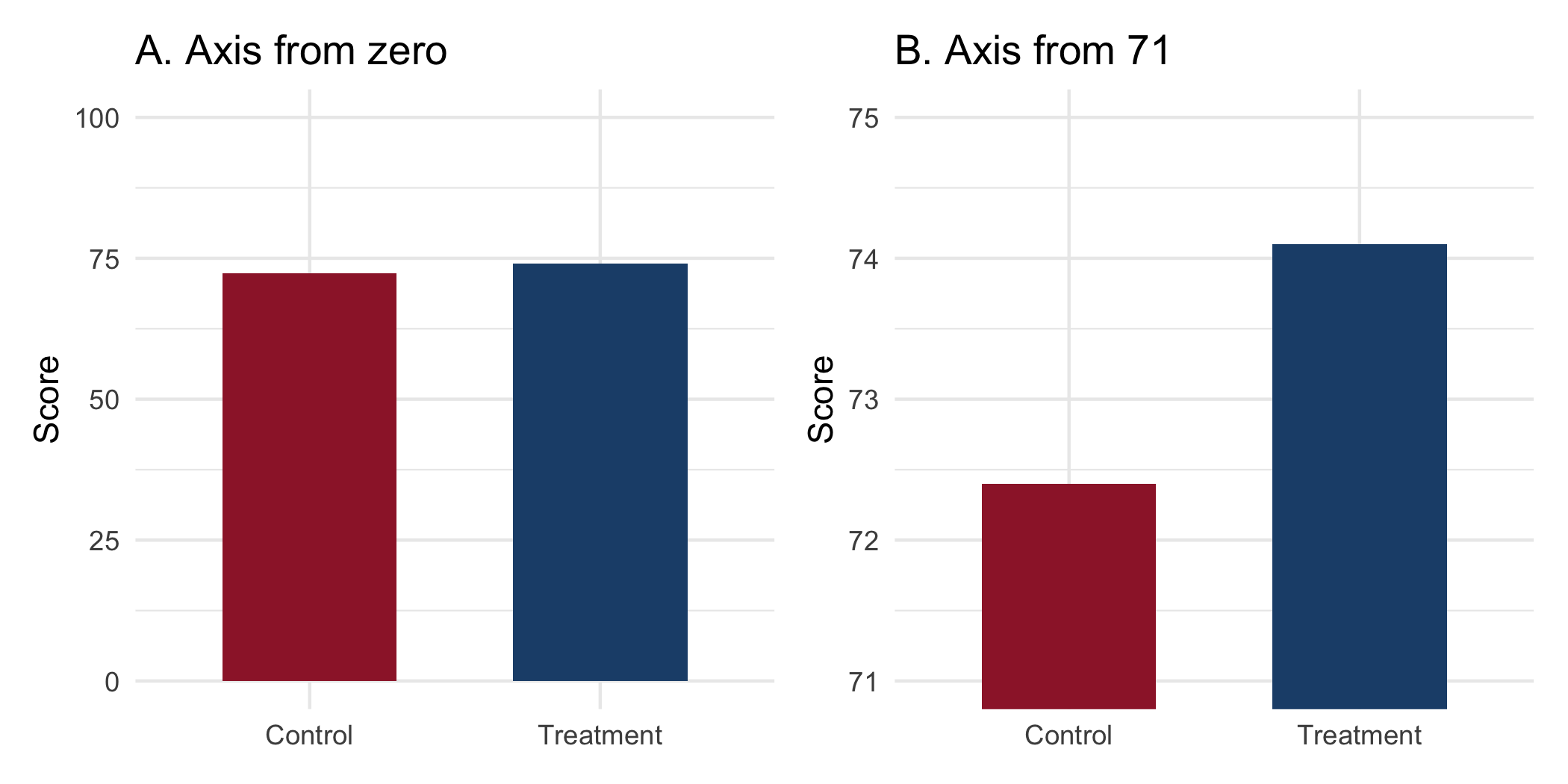
The difference is 1.7 points on a 100-point scale. Panel A tells you that. Panel B draws the treatment bar about 2.2 times as tall as the control bar. It suggests a difference the data do not contain, without printing a single incorrect value. There are three standard distortions.
The truncated axis. The rule is not ‘always start at zero’. For many quantities zero is meaningless (body temperature, calendar year, pH), and forcing it wastes the panel. The rule is that when the visual encoding is length or area, as in a bar chart, the baseline must be zero. The reader compares lengths, and a truncated bar’s length is not proportional to its value. For a point-and-interval plot, where the encoding is position, a truncated axis is legitimate and often necessary. The question is always what the reader’s eye is measuring.
Area for quantity. A map colored by which candidate won each county encodes land area, and land does not vote. A bubble whose radius is proportional to a count exaggerates it, because the eye reads area, which goes as the square of the radius. In biomedicine the recurring case is a map of disease counts that is really a map of where people live. The fix is a rate, a denominator, and a cartogram or population-weighted encoding.
The dual axis. Two series on two differently scaled y-axes can be made to cross, converge, or diverge at the analyst’s choice, because the relative scaling is arbitrary. Avoid dual axes. To compare two series, index them to a common baseline or use two panels. A language model asked to critique a described figure identifies a truncated baseline reliably. It is weaker on area encodings and denominators, which require knowing what the quantity means. Render the figure both ways, as above, and compare.
32.5.1 Exercises
- For the two means in Figure 32.3, find the axis floor at which the treatment bar is drawn exactly three times as tall as the control bar, and say what a reader would infer from that panel.
NoteSolution
floor_for_ratio <- function(ratio, low, high) {
  (ratio * low - high) / (ratio - 1)
}
floor_3 <- floor_for_ratio(3, d$mean[1], d$mean[2])
c(floor = floor_3,
  check = (d$mean[2] - floor_3) / (d$mean[1] - floor_3))
#> floor check
#> 71.55  3.00
Setting \((74.1 - f) = 3(72.4 - f)\) gives \(f = 71.55\). A reader of that panel would infer that treatment roughly triples the score, from a difference of 1.7 points on a 100-point scale. The floor needed is only about a point below the control mean, which is how easily a default axis range produces the distortion.
NoteCheck
Question. A forest plot of hazard ratios uses a horizontal axis from 0.5 to 2, not from zero. Is that a truncated-axis distortion?
Answer. No. The encoding is position, not length: each estimate is a point with an interval, and the reader compares positions against the reference line at 1. Starting at zero would waste the panel and compress the intervals. (A log scale is also the right choice for ratios, so that 0.5 and 2 sit equally far from 1.)
32.6 The overlapping-interval fallacy
The fourth failure is the one a biostatistician is most likely to commit personally. It is a technical error rather than a rhetorical one. The reasoning goes: the 95% confidence intervals for the two group means overlap, therefore the difference is not significant at the 5% level. This is wrong, and wrong in the direction of missing real effects. The interval for a difference depends on the standard error of the difference. That standard error is smaller than the sum of the two individual standard errors. Intervals for the two means can therefore overlap while the interval for their difference excludes zero. A demonstration, on synthetic data constructed to make the point clearly:
set.seed(18)

a <- rnorm(60, mean = 100, sd = 12)
b <- rnorm(60, mean = 105, sd = 12)

ci <- function(x) {
  m  <- mean(x)
  se <- sd(x) / sqrt(length(x))
  c(lower = m - 1.96 * se, mean = m, upper = m + 1.96 * se)
}

ci_tab <- rbind(group_a = ci(a), group_b = ci(b)) |> round(1)
ci_tab
#>         lower  mean upper
#> group_a  96.0  99.4 102.7
#> group_b 101.7 104.3 106.9

overlap_test <- t.test(b, a)
overlap_test
#>
#>  Welch Two Sample t-test
#>
#> data:  b and a
#> t = 2.289, df = 111.36, p-value = 0.02397
#> alternative hypothesis: true difference in means is not equal to 0
#> 95 percent confidence interval:
#>  0.6621209 9.1959712
#> sample estimates:
#> mean of x mean of y
#> 104.28772  99.35868
The two intervals overlap: group A reaches 102.7 and group B begins at 101.7. The two-sample test nonetheless rejects at the 5% level (\(p = 0.02\)). Anyone reading the overlap off a figure and concluding ‘no significant difference’ has reached the opposite conclusion from the one the data support.
The overlap here is about 1 point, which is deliberate. The fallacy does its damage in exactly this range, where the intervals barely overlap and the difference is real. As the difference grows, the intervals separate and the two readings agree. As it shrinks, the test stops rejecting and they agree again. The heuristic fails in the middle, where an analyst most wants guidance from the figure. Figure 32.4 shows the correct object: the interval for the difference, which answers the question actually asked.
means <- bind_rows(
  as_tibble_row(ci(a)) |> mutate(group = "A"),
  as_tibble_row(ci(b)) |> mutate(group = "B")
)

tt <- t.test(b, a)
diff <- tibble(
  group = "B - A",
  mean  = unname(diff(rev(tt$estimate))),
  lower = tt$conf.int[1],
  upper = tt$conf.int[2]
)

p_means <- ggplot(means, aes(mean, group)) +
  geom_pointrange(aes(xmin = lower, xmax = upper)) +
  labs(title = "A. Group means", x = "Score", y = NULL) +
  theme_minimal()

p_diff <- ggplot(diff, aes(mean, group)) +
  geom_pointrange(aes(xmin = lower, xmax = upper)) +
  geom_vline(xintercept = 0, linetype = "dashed",
             color = "#9d2235") +
  labs(title = "B. Difference", x = "Difference in score",
       y = NULL) +
  theme_minimal()

p_means + p_diff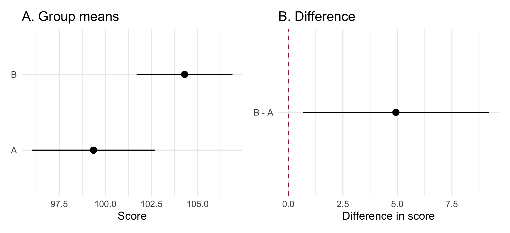
The practical consequences are two. When you report, give the interval for the contrast, not merely intervals for the arms, because the contrast is the estimand. When you review, treat any sentence of the form ‘the intervals overlapped, so the groups did not differ’ as an error, and say so.
32.6.1 Exercises
- Construct a dataset in which two group means have overlapping 95% intervals and a two-sample t-test rejects at the 5% level. State the largest overlap you can achieve while retaining significance, and explain the relationship between the standard error of a mean and the standard error of a difference.
NoteSolution
Build the groups deterministically rather than by sampling, so that the demonstration does not depend on the draw. Standardizing a random vector gives a group with exactly the mean and standard deviation you asked for:
set.seed(21)
n <- 60
exact <- function(mean, sd, n) {
  z <- as.numeric(scale(rnorm(n)))   # mean 0, sd 1 exactly
  mean + sd * z
}

g1 <- exact(100.00, 6, n)
g2 <- exact(102.63, 6, n)            # delta chosen below

ci <- function(x) mean(x) + c(-1, 1) * qt(0.975, length(x) - 1) *
                  sd(x) / sqrt(length(x))

round(ci(g1), 2)
#> [1]  98.45 101.55
round(ci(g2), 2)
#> [1] 101.08 104.18

tt <- t.test(g2, g1)
round(c(difference = mean(g2) - mean(g1),
        p = tt$p.value), 4)
#> difference          p
#>     2.6300     0.0179
round(as.numeric(tt$conf.int), 2)
#> [1] 0.46 4.80
The two per-group intervals overlap, the test rejects, and the interval for the difference excludes zero. Nothing here is contradictory; the three statements answer different questions.
The arithmetic explains the result and sets the window the delta above was chosen from. The standard error of one mean is \(s/\sqrt{n}\). The standard error of the difference of two independent means is \(\sqrt{s_1^2/n_1 + s_2^2/n_2}\), which for equal groups is \(\sqrt{2}\) times one group’s standard error, not twice it. Writing \(c \approx 2\) for the critical value at \(n = 60\):
- The two intervals overlap while \(\delta < 2c\,s/\sqrt{n} \approx 4.0\,s/\sqrt{n}\).
- The test rejects once \(\delta > c\sqrt{2}\,s/\sqrt{n} \approx 2.83\,s/\sqrt{n}\).
Any \(\delta\) between those two bounds gives both at once, and with \(s = 6\) and \(n = 60\) the window is roughly 2.19 to 3.10. The value 2.63 sits in the middle of it.
The largest overlap you can achieve is at the lower edge, where the test only just rejects:
overlap_at <- function(delta, n = 60, sd = 6) {
  set.seed(21)
  a <- exact(100, sd, n); b <- exact(100 + delta, sd, n)
  ca <- ci(a); cb <- ci(b)
  c(delta = delta,
    p = t.test(b, a)$p.value,
    overlap = unname(ca[2] - cb[1]))
}

sweep <- t(vapply(c(2.2, 2.4, 2.63, 2.8, 3.0, 3.2),
                  overlap_at, numeric(3))) |>
  round(3)
sweep
#>      delta     p overlap
#> [1,]  2.20 0.047    0.90
#> [2,]  2.40 0.030    0.70
#> [3,]  2.63 0.018    0.47
#> [4,]  2.80 0.012    0.30
#> [5,]  3.00 0.007    0.10
#> [6,]  3.20 0.004   -0.10
Every row here rejects, so read the first: at \(\delta = 2.2\) the test gives \(p = 0.047\) and the intervals still overlap by 0.9 units. That is the widest overlap compatible with significance in this design. Reducing \(\delta\) further loses the rejection. Going the other way, the overlap shrinks steadily and turns negative by \(\delta = 3.2\), where the intervals have separated. The sweep also confirms the bounds computed above. The lower edge sits just under 2.2 and the upper just over 3.0, against the predicted 2.19 and 3.10.
Reading significance off the overlap on the left-hand panel of Figure 32.4 is therefore not a conservative approximation. It is a test with the wrong standard error, and it fails in the direction of declaring ‘no difference’ when there is one.
NoteCheck
Question. Two arms’ 95% intervals do not overlap. May you conclude that the difference is significant at the 5% level?
Answer. Yes, for two independent estimates. Non-overlap is a stricter criterion than the test, so it errs only toward missing real differences, never toward declaring false ones. The fallacy runs one way only, which is why it is easy to miss. The rule ‘overlap means no difference’ sounds like the mirror image of a correct rule, but it is not.
32.7 Unrepresentative samples
The fifth failure is the one whose costs fall on people who are not in the room, and often not in the data. It is the failure of fair representation. It is why a competent statistician asks who a sample contains before, not after, generalizing from it. Once again, no number is false. The error is the unstated step from ‘this holds in the sample’ to ‘this holds’. That step is taken when the sample and the target are not the same population and no one has said so. This book’s own source material shows the mechanism. The survey behind the team-science reading drew respondents who were 82.8% White. Its authors state plainly that their conclusions may not transport to a more diverse workforce (Slade et al., 2023). Their disclosure is the practice to copy, and the skew is the hazard it warns of.
A sample is evidence about the population it was drawn from, and no other. Consider a drug trial that enrolls at academic medical centers, among patients who can attend visits every two weeks. Its sample skews toward the younger, the insured, the urban, and those without other illnesses. Applied to the older, rural patient with several illnesses to whom the drug will be prescribed, its estimate is an extrapolation (Rothwell, 2005). Adjusting for age does not repair this, for the same reason it did not repair the volunteer cohort. The groups differ along dimensions no covariate list enumerates.
Under-representation costs a subgroup both precision and bias. When a subgroup is a small fraction of the sample, its estimate is imprecise. An effect specific to that subgroup is therefore the effect you are least able to detect. If the effect genuinely differs there, the pooled estimate, dominated by the majority, is also biased for them. A result reported as though it applied to everyone fails exactly the people the sample underweighted. It fails them silently, because the interval on the pooled estimate looks reassuringly tight.
A model learns the sample’s inequities and returns them as findings. Some analyses feed a decision rule (a risk score, an eligibility threshold, a resource-allocation model). There, a biased training sample propagates the bias at scale. The standard example is a health-system algorithm that used prior health-care spending as a proxy for health need. Less had historically been spent on Black patients at equal levels of illness. The algorithm therefore systematically understated their need (Obermeyer et al., 2019). Every number was correctly computed. The proxy was the error, and only someone asking what the variable stood for could have caught it.
The necessary practices are cheap, and Table 32.6 lists them.
| Practice | What to do | Example sentence or check |
|---|---|---|
| Report who is in the sample beside who the result is for | Table 1 by demographic group; name the populations to which the estimate does and does not transport | ‘Our cohort was 91% White and privately insured; generalization to other populations is unestablished.’ |
| Pre-specify the subgroups you are powered to examine | Label the rest exploratory (Chapter 26) | A subgroup you were not powered for yields an imprecise estimate, not an absence of effect |
| Ask what a decision variable is a proxy for | Before a predictor enters a model that acts on people, check whether it encodes a protected characteristic and whether errors are borne equally | Spending as a proxy for need |
| Make the artifact readable by every reader | Color-blind-safe palettes, verified before publication (Chapter 20) | Red versus green is illegible to roughly 8% of men |
WarningPitfall
A subgroup row in Table 1 is reported; its uncertainty is not. A Table 1 that lists a few dozen patients in a group invites a reader to treat the group as studied. A subgroup estimate for a few dozen patients has an interval so wide that it can neither show nor exclude any plausible effect. A report that says ‘no difference was observed in this group’ has converted imprecision into a finding. Report the interval, or say that the group was too small to examine.
32.7.1 Exercises
- Using the HF-HOME files, compute for each race category the number of randomized patients and the half-width of the 95% interval for the risk difference between arms among ascertained patients. Which groups could support any subgroup claim?
NoteSolution
hf_dir <- file.path("..", "data", "raw_data", "hfhome")
read_hf <- function(file) {
  read_csv(file.path(hf_dir, file),
           col_types = cols(patient_id = "c", .default = "?"))
}

hf <- read_hf("randomization.csv") |>
  select(patient_id, arm) |>
  left_join(read_hf("outcomes.csv") |>
              select(patient_id, ascertained, event_30d),
            by = "patient_id", relationship = "one-to-one",
            unmatched = "error") |>
  left_join(read_hf("demographics.csv") |> select(patient_id, race),
            by = "patient_id", relationship = "one-to-one",
            unmatched = "error")
stopifnot(nrow(hf) == nrow(read_hf("randomization.csv")))

by_race <- hf |>
  filter(ascertained) |>
  group_by(race, arm) |>
  summarize(n = n(), p = mean(event_30d), .groups = "drop") |>
  group_by(race) |>
  summarize(patients = sum(n),
            half_width = 100 * qnorm(0.975) *
              sqrt(sum(p * (1 - p) / n)),
            .groups = "drop") |>
  arrange(patients)
by_race
#> # A tibble: 7 × 3
#>   race                                      patients half_width
#>   <chr>                                        <int>      <dbl>
#> 1 Native Hawaiian or Other Pacific Islander       24      37.9
#> 2 American Indian or Alaska Native                27      36.4
#> 3 Multiple                                        81      17.9
#> 4 Asian                                          249      11.1
#> 5 Not reported                                   315       8.89
#> 6 Black or African American                      338       8.91
#> 7 White                                         1235       4.57
The smallest groups have half-widths of about 38 points, against an overall effect of a few points. They can support no subgroup claim at all, in either direction. Only the largest group, White, has a half-width (4.6 points) below the 5-point reduction the trial was designed to detect. It does so only just, because it holds about half the trial. The honest report gives the composition and says that the trial was not designed to estimate effects by race. It names the groups too small to examine, rather than reporting ‘no difference’ in each.
NoteCheck
Question. A risk model is trained on a health system’s records and validated with excellent overall discrimination. What question does the overall validation leave unanswered?
Answer. Whether the model’s errors are borne equally. Overall discrimination is dominated by the majority of the sample. A model can rank well overall while systematically under- or over-predicting for a group. This is especially likely if a predictor is a proxy for something other than what it is named for. Validate by group, and ask what each predictor stands for, before the model acts on anyone.
32.8 Rules of thumb
- Habit 11: lead with the answer, and match the verb to the design. Observational studies license association; when the question is causal, state it and its assumptions openly.
- Habit 5: pre-specify, then tag. A dated plan is what separates a reported exploratory analysis from HARKing, and a powered subgroup from an imprecise one.
- Habit 8: a bug that produces a plausible number is the expensive kind. A truncated axis, an overlap read as a test, and a proxy variable all produce plausible pictures; ask what the reader’s eye, the test, and the variable are measuring.
32.9 Cumulative practice
- Cumulative (uses Chapter 20 and Chapter 33). Draw HF-HOME’s primary result twice: once as two bars of observed risk with the y-axis from 20% to 24.5% and no intervals, and once as the risk difference with its 95% interval against zero and the 5-point minimum clinically important difference. Write one sentence a reader would take from each.
-
On your own work (no key). Take the discussion section of a paper you have co-authored. Run
flag_causal()on it, then, for every flagged sentence, state the design that would license it and the design you actually had, and rewrite any that fail.
NoteSolution to exercise 6
arm_risk <- hf |>
  filter(ascertained) |>
  group_by(arm) |>
  summarize(n = n(), risk = mean(event_30d), .groups = "drop") |>
  mutate(arm = factor(arm, levels = c("Usual care", "Home health"))) |>
  arrange(arm)

rd <- 100 * (arm_risk$risk[1] - arm_risk$risk[2])
se <- 100 * sqrt(sum(arm_risk$risk * (1 - arm_risk$risk) / arm_risk$n))
rd_tab <- tibble(label = "Usual care minus home health", est = rd,
                 lower = rd - qnorm(0.975) * se,
                 upper = rd + qnorm(0.975) * se)

p_bad <- ggplot(arm_risk, aes(arm, 100 * risk)) +
  geom_col(width = 0.6) +
  coord_cartesian(ylim = c(20, 24.5)) +
  labs(x = NULL, y = "30-day risk (%)",
       title = "A. Home health works?") +
  theme_minimal()

p_good <- ggplot(rd_tab, aes(est, label)) +
  geom_vline(xintercept = 0) +
  geom_vline(xintercept = 5, linetype = "dashed") +
  geom_pointrange(aes(xmin = lower, xmax = upper)) +
  labs(x = "Risk difference (points)", y = NULL,
       title = "B. Inconclusive") +
  theme_minimal()

p_bad + p_good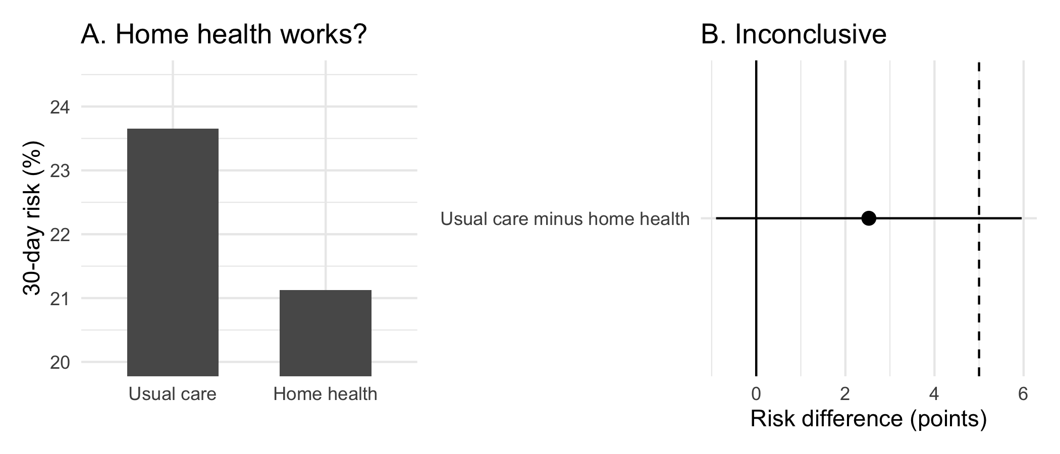
Panel A says ‘home health cut readmissions sharply’; panel B says ‘the trial cannot distinguish no effect from a reduction of about 6 points’. Both use the same 2,269 ascertained patients and print no false number. Panel A commits two of this chapter’s failures at once: a truncated length encoding, and a pair of arm estimates shown without the contrast that is the estimand.
32.10 Cheat sheet
| Failure | Ask | Do |
|---|---|---|
| Aggregation harm | Would the people in it be surprised? | De-identify, or do not assemble |
| Misconduct and QRPs | Was this decision dated before the data? | Pre-specify; disclose every exclusion and analysis |
| Causal overclaiming | Does the design license the verb? | Rewrite to the licensed register; state causal assumptions openly |
| Visual misrepresentation | What is the reader’s eye measuring? | Zero baseline for length; no dual axes |
| Overlapping intervals | Is the claim about the contrast? | Report and plot the interval for the difference |
| Unrepresentative sample | To whom does the estimate transport? | Report composition; name the populations it does not cover |
32.11 Further reading
- (American Statistical Association, 2022), the profession’s own statement of what this chapter argues, and the document to cite when you decline.
- (Hernán, 2018), on stating causal questions openly rather than hiding them behind associational language.
- (Obermeyer et al., 2019), the health-system algorithm whose proxy variable encoded and propagated racial bias at scale.
32.12 Prerequisites answers
- Because the harm of aggregation differs from the harm of disclosure. Each individual disclosed a fact to an audience of their choosing, in a context they understood. Assembling those disclosures into a single searchable, permanent, downloadable artifact, with identifiers attached, does something none of them chose. The aggregate can reveal what no individual datum did, for example by linking a health disclosure in one forum to an employer named in another. This is the joint-distribution phenomenon that makes quasi-identifiers dangerous in Chapter 4, arriving from the other direction. The test is not ‘was each item public’ but ‘would the people in the dataset be surprised to find themselves in it’.
- No. The confidence interval for the difference depends on the standard error of the difference, which is smaller than the sum of the two individual standard errors. Two means can therefore have overlapping intervals while the interval for their difference excludes zero and the two-sample test rejects. The error runs in the direction of missing real effects. Report and inspect the interval for the contrast, which is the estimand.
- (Any three of:) a truncated axis on a length-encoded chart, so that a 1.7-point difference on a 100-point scale fills the panel; encoding a quantity as area, including a map colored by land rather than by population, or a bubble whose radius rather than area is proportional to the count; a dual axis, whose relative scaling is an arbitrary choice that can make two series appear to converge or diverge; omitting the uncertainty, so that a point estimate invites more confidence than it has earned; and choosing a denominator that flatters the conclusion. None requires printing a false number.