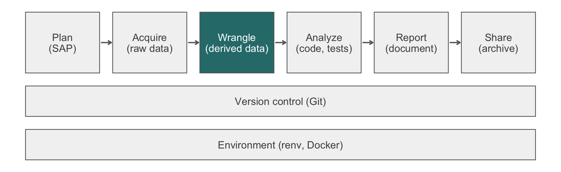
18 Joining and Reshaping
A join can fail in two ways, and neither raises an error. First, it can drop rows. This happens when a key present on one side is absent on the other. The analysis then proceeds on a smaller, and possibly different, cohort than the one the methods section describes. Second, it can multiply rows. This happens when a key that should be unique is not. A patient then contributes several times to an estimate that assumed one contribution. The first failure shrinks the denominator, and the second corrupts the standard errors. In both cases the data frame looks like the one you wanted. Simple arithmetic catches both. We state how many rows the result should have, and check that against how many it does.
Only connect.
E. M. Forster, Howards End (1910)
NoteIn this chapter
Reading time. About 25 minutes.
You’ll need. Chapter 15 for the single-table verbs and pivot_longer()/pivot_wider(), and Chapter 16 for column types. The code uses:
You’ll be able to.
- Choose the join that answers a stated question and predict its row count before you run it.
- Declare the expected relationship and the unmatched behavior, so that the join refuses data that violate them.
- Audit keys for uniqueness, type, and coverage with
count()andanti_join()before joining. - Reshape and stack sources with different conventions so that a later join cannot multiply rows.
Outline.
NoteSkip ahead?
If these answers come quickly, skip to the next chapter. The answers are in Section 18.10.
- What is the difference in row count between
inner_join()andleft_join()when the right table is missing some keys that appear in the left table? - What does
anti_join()return, and in a biomedical cleanup workflow, what question does it answer? - Given two tables each with a
patient_idcolumn and a many-to-one relationship (many rows per patient in table A, one row per patient in table B), how do you attach the table-B row to every table-A row?
18.1 Choosing a join
Almost every biostatistical project joins tables: demographics to outcomes, labs to medications, clinical data to imaging indices. The operation is one function call. The difficulty lies in the question the join is meant to answer, and in what the keys actually contain. The generic tour of the two-table verbs is in R for Data Science (Wickham et al., 2023, ch. 19). In this chapter we keep to the judgments that a clinical dataset requires.
18.1.1 The _join family
dplyr’s two-table verbs:
| Function | Returns |
|---|---|
inner_join |
Rows with a match in both |
left_join |
All rows from x, NA in y columns where no match |
right_join |
All rows from y, NA in x columns where no match |
full_join |
All rows from both, NA in non-matching columns |
semi_join |
Rows of x with a match in y (no y cols) |
anti_join |
Rows of x with no match in y
|
semi_join and anti_join are filtering joins. They filter x based on y without adding y’s columns. The other four are mutating joins, which add columns.1 The choice among the mutating joins comes down to two questions, shown in Figure 18.2. Do you want to keep rows that fail to match? If so, from which side?
1 In pandas, the four mutating joins are one call, x.merge(y, on="id", how=...) with how set to "inner", "left", "right", or "outer". The filtering joins have no merge equivalent and are written with isin(), for example x[~x["id"].isin(y["id"])] for an anti-join.
flowchart TD
  Q1{"Keep rows with<br/>no match?"}
  Q1 -->|"No"| INNER["inner_join"]
  Q1 -->|"Yes"| Q2{"Unmatched from<br/>which side?"}
  Q2 -->|"Left x"| LEFT["left_join"]
  Q2 -->|"Right y"| RIGHT["right_join"]
  Q2 -->|"Both"| FULL["full_join"]
The question determines the join:
| Question | Join |
|---|---|
| Patients with both demographics and an outcome | inner_join |
| All patients, with their outcomes if any |
left_join, demographics on the left |
| Patients with demographics but no outcome | anti_join |
| All patients from both files, even those in only one | full_join |
18.1.2 Row counts on a toy example
The dplyr package ships two toy tables, band_members and band_instruments, that make the row-count differences concrete. Before you run the chunk, predict how many rows each join returns.
library(dplyr)

band_members
#> # A tibble: 3 × 2
#>   name  band
#>   <chr> <chr>
#> 1 Mick  Stones
#> 2 John  Beatles
#> 3 Paul  Beatles
band_instruments
#> # A tibble: 3 × 2
#>   name  plays
#>   <chr> <chr>
#> 1 John  guitar
#> 2 Paul  bass
#> 3 Keith guitar

inner_join(band_members, band_instruments, by = "name")  # John, Paul
#> # A tibble: 2 × 3
#>   name  band    plays
#>   <chr> <chr>   <chr>
#> 1 John  Beatles guitar
#> 2 Paul  Beatles bass
left_join(band_members, band_instruments, by = "name")   # + Mick (NA)
#> # A tibble: 3 × 3
#>   name  band    plays
#>   <chr> <chr>   <chr>
#> 1 Mick  Stones  <NA>
#> 2 John  Beatles guitar
#> 3 Paul  Beatles bass
full_join(band_members, band_instruments, by = "name")   # + Keith (NA)
#> # A tibble: 4 × 3
#>   name  band    plays
#>   <chr> <chr>   <chr>
#> 1 Mick  Stones  <NA>
#> 2 John  Beatles guitar
#> 3 Paul  Beatles bass
#> 4 Keith <NA>    guitar
anti_join(band_members, band_instruments, by = "name")   # Mick only
#> # A tibble: 1 × 2
#>   name  band
#>   <chr> <chr>
#> 1 Mick  Stones
TipVerification
Write your predictions down as assertions. The chunk prints nothing when every prediction holds, and stops at the first one that does not.
18.1.3 Exercises
- Use each of
inner_join,left_join,full_join, andanti_joinwith the built-indplyr::band_membersanddplyr::band_instrumentsto produce four different tibbles. Write one sentence per result.
NoteSolution
inner_join(band_members, band_instruments, by = "name")
#> # A tibble: 2 × 3
#>   name  band    plays
#>   <chr> <chr>   <chr>
#> 1 John  Beatles guitar
#> 2 Paul  Beatles bass
left_join(band_members, band_instruments, by = "name")
#> # A tibble: 3 × 3
#>   name  band    plays
#>   <chr> <chr>   <chr>
#> 1 Mick  Stones  <NA>
#> 2 John  Beatles guitar
#> 3 Paul  Beatles bass
full_join(band_members, band_instruments, by = "name")
#> # A tibble: 4 × 3
#>   name  band    plays
#>   <chr> <chr>   <chr>
#> 1 Mick  Stones  <NA>
#> 2 John  Beatles guitar
#> 3 Paul  Beatles bass
#> 4 Keith <NA>    guitar
anti_join(band_members, band_instruments, by = "name")
#> # A tibble: 1 × 2
#>   name  band
#>   <chr> <chr>
#> 1 Mick  Stones
inner_join keeps only John and Paul, who appear in both. left_join keeps all three band members, giving Mick an NA instrument. full_join keeps Keith as well, giving him an NA band. anti_join returns Mick alone, the band member with no instrument row, and adds no columns.
NoteCheck
Question. A collaborator asks for ‘the patients in the demographics file who have no outcome record’. Which join answers this, and how many columns of the outcome table does the result carry?
Answer. anti_join(demographics, outcomes, by = "patient_id"). It is a filtering join, so it carries none of the outcome table’s columns. It returns rows of demographics only. A left_join followed by filter(is.na(outcome)) gives the same patients, but with two drawbacks. It adds columns you then have to drop. It also misreads a patient whose outcome record exists with a missing value as a patient with no record.
18.2 Cardinality: when a join multiplies rows
18.2.1 Many-to-many joins
A many-to-many join occurs when both tables have duplicate keys. Each row in the left can match several rows in the right, and the reverse. The result is the product of the matches for each key.
library(dplyr)

a <- tibble(id = c(1, 1, 2), x = c("a", "b", "c"))
b <- tibble(id = c(1, 1, 2), y = c("p", "q", "r"))

# Five rows, not three: each id-1 in a joins each id-1 in b, giving
# four, plus the single id-2 match. dplyr warns because this is
# usually a key error rather than an intention.
inner_join(a, b, by = "id")
#> Warning in inner_join(a, b, by = "id"): Detected an unexpected many-to-many relationship between `x` and `y`.
#> ℹ Row 1 of `x` matches multiple rows in `y`.
#> ℹ Row 1 of `y` matches multiple rows in `x`.
#> ℹ If a many-to-many relationship is expected, set `relationship =
#>   "many-to-many"` to silence this warning.
#> # A tibble: 5 × 3
#>      id x     y
#>   <dbl> <chr> <chr>
#> 1     1 a     p
#> 2     1 a     q
#> 3     1 b     p
#> 4     1 b     q
#> 5     2 c     r
dplyr 1.1.0 and later warns by default. Take the warning seriously. On a key that should be unique, it means rows have multiplied. Do not silence it. Instead, declare the relationship you expect:
# explicit; no warning, even with duplicates
inner_join(a, b, by = "id", relationship = "many-to-many")
#> # A tibble: 5 × 3
#>      id x     y
#>   <dbl> <chr> <chr>
#> 1     1 a     p
#> 2     1 a     q
#> 3     1 b     p
#> 4     1 b     q
#> 5     2 c     r

# errors if duplicates exist on either side
inner_join(a, b, by = "id", relationship = "one-to-one")
#> Error in `inner_join()`:
#> ! Each row in `x` must match at most 1 row in `y`.
#> ℹ Row 1 of `x` matches multiple rows in `y`.
18.2.2 Declaring the relationship
The common case is many-to-one: several visits per patient, and one demographics row per patient. The rest of the chapter uses the three small tables below. P004 appears in visits but not in demographics. The audits in Section 18.3 are designed to catch this kind of gap.
demographics <- tibble(
  patient_id = c("P001", "P002", "P003"),
  age        = c(64, 71, 52),
  sex        = c("F", "M", "F")
)
visits <- tibble(
  visit_id   = sprintf("V%02d", 1:6),
  patient_id = c("P001", "P001", "P002", "P002", "P003", "P004"),
  sbp        = c(148, 141, 155, 149, 132, 139)
)
labs <- tibble(
  visit_id  = c("V01", "V01", "V02", "V03"),
  test_code = c("HGB", "CRE", "HGB", "HGB"),
  value     = c(13.1, 0.9, 13.4, 11.8)
)

demographics
#> # A tibble: 3 × 3
#>   patient_id   age sex
#>   <chr>      <dbl> <chr>
#> 1 P001          64 F
#> 2 P002          71 M
#> 3 P003          52 F
visits
#> # A tibble: 6 × 3
#>   visit_id patient_id   sbp
#>   <chr>    <chr>      <dbl>
#> 1 V01      P001         148
#> 2 V02      P001         141
#> 3 V03      P002         155
#> 4 V04      P002         149
#> 5 V05      P003         132
#> 6 V06      P004         139
labs
#> # A tibble: 4 × 3
#>   visit_id test_code value
#>   <chr>    <chr>     <dbl>
#> 1 V01      HGB        13.1
#> 2 V01      CRE         0.9
#> 3 V02      HGB        13.4
#> 4 V03      HGB        11.8
visits |>
left_join(demographics, by = "patient_id",
relationship = "many-to-one")
#> # A tibble: 6 × 5
#> visit_id patient_id sbp age sex
#> <chr> <chr> <dbl> <dbl> <chr>
#> 1 V01 P001 148 64 F
#> 2 V02 P001 141 64 F
#> 3 V03 P002 155 71 M
#> 4 V04 P002 149 71 M
#> 5 V05 P003 132 52 F
#> 6 V06 P004 139 NA <NA>
# errors if a patient_id appears more than once in demographicsThe assertion catches the data-quality bug at the join site, where it is easiest to debug. Without it, the bug would appear three scripts later as a standard error that is too small.
WarningPitfall
A one-to-many join multiplies rows without a warning. dplyr warns only when keys repeat on both sides. Suppose each visit key is unique, and a patient appears twice in demographics (a re-consent appended rather than replaced). Then left_join(visits, demographics) quietly returns an extra row for every visit of that patient. Only relationship = "many-to-one" turns this into an error.
18.2.3 Exercises
- Construct a scenario where an unintended many-to-many join duplicates rows. Write an assertion that catches the duplication before downstream analysis.
NoteSolution
# demographics has a duplicated patient, perhaps from a
# re-consent that was appended rather than replaced
demo_dup <- tibble(patient_id = c("P001", "P001", "P002"),
                   age = c(64, 65, 71))
vis <- tibble(patient_id = c("P001", "P002"), sbp = c(148, 155))

# the silent version: two rows become three
left_join(vis, demo_dup, by = "patient_id")
#> # A tibble: 3 × 3
#>   patient_id   sbp   age
#>   <chr>      <dbl> <dbl>
#> 1 P001         148    64
#> 2 P001         148    65
#> 3 P002         155    71

# the assertion, before anything downstream runs
stopifnot(!anyDuplicated(demo_dup$patient_id))
#> Error:
#> ! !anyDuplicated(demo_dup$patient_id) is not TRUE
The join itself does not fail. It quietly returns more rows than it received, and because vis has unique keys, dplyr does not even warn. The stopifnot() fails loudly, which is the behavior you want. Declaring relationship = "many-to-one" on the join achieves the same thing at the point of use.
NoteCheck
Question. You join visits (10,000 rows) to demographics (1,000 patients) on patient_id. The result has 12,500 rows. What likely happened, and how do you find out?
Answer. The demographics table has duplicate patient_id values, and each duplicate creates extra rows in the join output. A clean many-to-one join returns 10,000 rows, one per visit. The 2,500 extra rows are the visits of patients with more than one demographics record. Diagnose with:
Fix the duplication at its source. The tempting shortcut is distinct(patient_id, .keep_all = TRUE). It keeps whichever row for each patient happens to come first. That is, it chooses a record by file order rather than by any rule. If the duplicates disagree on age or sex, which one survives is an accident. If de-duplication is right, state the rule in code (the most recent record, say, with slice_max() on a date column). Adding relationship = "many-to-one" to the join catches the problem at the join site.
18.3 Keys and referential integrity
A join that returns the number of rows you predicted usually did what you meant. A join that returns ‘about the right number’ is where the bugs are usually found. The checks below run before the analytic join and take seconds.
18.3.1 Auditing keys before the join
Two CRF (case report form) files that should cover the same patients usually do not match exactly. anti_join() lists the patients on one side that are absent from the other. It is the quickest way to find missing records, ID typos, or a cohort mismatch.
# uniqueness of keys
demographics |> distinct(patient_id) |> nrow()
#> [1] 3
demographics |> nrow()
#> [1] 3
# These should match for one-row-per-patient

# stopifnot for assertion
stopifnot(!any(duplicated(demographics$patient_id)))

# anti-join audit
visits |> anti_join(demographics, by = "patient_id") |>
  distinct(patient_id)
#> # A tibble: 1 × 1
#>   patient_id
#>   <chr>
#> 1 P004
# patients in visits with no demographics row
assertthat and assertr provide more elaborate assertions. For most work, stopifnot() plus anti_join() audits cover the cases.
18.3.2 Composite keys
When no single column identifies a row, name every column of the key:
reference_ranges <- tibble(
  test_code = c("HGB", "HGB", "CRE"),
  sex       = c("F", "M", "F"),
  age_group = c("50-70", "50-70", "50-70"),
  lower     = c(12.0, 13.5, 0.6),
  upper     = c(15.5, 17.5, 1.1)
)

labs |>
  left_join(visits, by = "visit_id") |>
  left_join(demographics, by = "patient_id") |>
  mutate(age_group = "50-70") |>
  left_join(reference_ranges,
            by = c("test_code", "sex", "age_group"))
#> # A tibble: 4 × 10
#>   visit_id test_code value patient_id   sbp   age sex   age_group lower upper
#>   <chr>    <chr>     <dbl> <chr>      <dbl> <dbl> <chr> <chr>     <dbl> <dbl>
#> 1 V01      HGB        13.1 P001         148    64 F     50-70      12    15.5
#> 2 V01      CRE         0.9 P001         148    64 F     50-70       0.6   1.1
#> 3 V02      HGB        13.4 P001         141    64 F     50-70      12    15.5
#> 4 V03      HGB        11.8 P002         155    71 M     50-70      13.5  17.5
18.3.3 Key types and representation
Document the canonical form of every identifier (character, with leading zeros, upper case) and check it on every read. dplyr refuses to join a character key to a numeric one. That failure is easy to see. The failure that is hard to see is two character keys that spell the same patient differently.
WarningPitfall
Lost leading zeros match nothing, and the row count does not move. If one file was read with patient_id as a number and later converted with as.character(), "001" has become "1". A left_join on that key returns every row of the left table, which is the count you expected. However, every right-hand column is NA. Read identifiers as character from the start (col_types = cols(patient_id = col_character())).
18.3.4 Aside: updating a table by key with rows_*
The rows_* verbs update one table from another by key, and they enforce key integrity as they go. They suit updating a master patient list from a new extract.
target <- tibble(id = 1:3, value = c("a", "b", NA))
source <- tibble(id = 3:4, value = c("c", "d"))

# insert new rows; error on key collision
rows_insert(target, source, by = "id")
#> Error in `rows_insert()`:
#> ! `y` can't contain keys that already exist in `x`.
#> ℹ The following rows in `y` have keys that already exist in `x`: `c(1)`.
#> ℹ Use `conflict = "ignore"` if you want to ignore these `y` rows.

# update existing rows; error if key not in target
rows_update(target, source, by = "id")
#> Error in `rows_update()`:
#> ! `y` must contain keys that already exist in `x`.
#> ℹ The following rows in `y` have keys that don't exist in `x`: `c(2)`.
#> ℹ Use `unmatched = "ignore"` if you want to ignore these `y` rows.

# upsert: insert new, update existing
rows_upsert(target, source, by = "id")
#> # A tibble: 4 × 2
#>      id value
#>   <int> <chr>
#> 1     1 a
#> 2     2 b
#> 3     3 c
#> 4     4 d

# patch: only update where target has NA; id 4 is not in target,
# so it must be ignored explicitly
rows_patch(target, source, by = "id", unmatched = "ignore")
#> # A tibble: 3 × 2
#>      id value
#>   <int> <chr>
#> 1     1 a
#> 2     2 b
#> 3     3 c
rows_upsert adds new patients and updates existing ones. rows_patch fills in missing values without overwriting existing ones.
18.3.5 Exercises
- Use
rows_upsertto merge two cohorts with overlapping patients (some new, some updated). Verify the result has the expected number of rows.
NoteSolution
cohort_1 <- tibble(patient_id = c("P001", "P002"),
                   status = c("enrolled", "enrolled"))
cohort_2 <- tibble(patient_id = c("P002", "P003"),
                   status = c("withdrawn", "enrolled"))

merged <- rows_upsert(cohort_1, cohort_2, by = "patient_id")
merged
#> # A tibble: 3 × 2
#>   patient_id status
#>   <chr>      <chr>
#> 1 P001       enrolled
#> 2 P002       withdrawn
#> 3 P003       enrolled

# two originals plus one genuinely new patient
stopifnot(nrow(merged) == 3)
P002 is updated in place rather than duplicated, and P003 is inserted. The row count distinguishes an upsert from an accidental bind_rows(). The latter would have produced four rows and two conflicting records for P002.
NoteCheck
Question. You left_join a 500-row visits table to a demographics table and get 500 rows back, which is what you expected. A colleague says this proves nothing. Are they right?
Answer. They are. A row count matching your expectation rules out duplication and rules out nothing else. Every patient_id in visits could have failed to match, and left_join would still return exactly 500 rows, each with NA in every demographics column. The lost-leading-zeros case above does exactly this.
The count does not catch this, but two other checks do. First, count the NAs in a column that came from the right-hand table. The count should be zero if every visit has demographics. Second, run the anti-join:
An empty result means every key matched. A result listing every patient means the join silently did nothing. nrow() is a structural check, in the sense Chapter 27 gives that term, and structural checks can pass on wrong answers.
18.4 Reshaping and stacking sources
Some joins need wide data and others need long data. Chapter 15 covers pivot_longer() and pivot_wider(). When several sources hold alternative measurements of the same kind, the usual pattern is:
- Convert each source to long format with consistent column names.
- Stack the sources with
bind_rows()rather than joining them. - Pivot wide for the modeling step.
For two CRF files from sites A and B with different column conventions (display-only; the files are hypothetical):
a_long <- read_csv("siteA.csv") |>
  clean_names() |>
  rename(bp_systolic = systolic_bp) |>
  pivot_longer(starts_with("bp_"), names_to = "measure")

b_long <- read_csv("siteB.csv") |>
  clean_names() |>
  pivot_longer(matches("^(bp|sbp|dbp)_"), names_to = "measure")

combined <- bind_rows(a_long, b_long)
bind_rows() stacks tables. bind_cols() places tables side by side by position. That is rarely correct for clinical data, because nothing checks that row 12 of one table is the same patient as row 12 of the other. When the tables share a key, join on it.
18.4.1 Exercises
- Two wide tables represent patient visits at sites A and B with different column-name conventions. Reshape both to long and stack them so that downstream analysis treats them uniformly.
NoteSolution
library(tidyr)

site_a <- tibble(patient_id = "A01",
                 systolic_bp = 148, diastolic_bp = 88)
site_b <- tibble(patient_id = "B01",
                 sbp_1 = 155, dbp_1 = 91)

a_long <- site_a |>
  rename(bp_systolic = systolic_bp, bp_diastolic = diastolic_bp) |>
  pivot_longer(starts_with("bp_"), names_to = "measure")

b_long <- site_b |>
  rename(bp_systolic = sbp_1, bp_diastolic = dbp_1) |>
  pivot_longer(starts_with("bp_"), names_to = "measure")

bind_rows(a_long, b_long, .id = "site")
#> # A tibble: 4 × 4
#>   site  patient_id measure      value
#>   <chr> <chr>      <chr>        <dbl>
#> 1 1     A01        bp_systolic    148
#> 2 1     A01        bp_diastolic    88
#> 3 2     B01        bp_systolic    155
#> 4 2     B01        bp_diastolic    91
Renaming to a shared vocabulary before the pivot is what makes bind_rows() safe. Stacking first and reconciling after leaves you matching on strings that do not agree.
NoteCheck
Question. The long labs table has one row per visit and test. You join it directly to visits on visit_id. What relationship is that, and what happens to a later model that expects one row per visit?
Answer. One-to-many: a visit with two tests appears twice. Any per-visit model then counts that visit twice. Pivot labs wide first, to one row per visit, and declare relationship = "one-to-one" on the join. The worked example below does both.
18.5 Worked example: a multi-source patient cohort
The script below runs against the three fixture tables shown earlier. They are written out as files, so that the script reads them as it would read a real export. P004, who has visits but no demographics row, is planted deliberately, so the audit warns once.
library(tidyverse)
#> ── Attaching core tidyverse packages ──────────────────────── tidyverse 2.0.0 ──
#> ✔ forcats   1.0.1     ✔ readr     2.2.0
#> ✔ ggplot2   4.0.3     ✔ stringr   1.6.0
#> ✔ lubridate 1.9.5     ✔ tibble    3.3.1
#> ✔ purrr     1.2.2
#> ── Conflicts ────────────────────────────────────────── tidyverse_conflicts() ──
#> ✖ dplyr::filter() masks stats::filter()
#> ✖ dplyr::lag()    masks stats::lag()
#> ℹ Use the conflicted package (<http://conflicted.r-lib.org/>) to force all conflicts to become errors
library(janitor)
#>
#> Attaching package: 'janitor'
#>
#> The following objects are masked from 'package:stats':
#>
#>     chisq.test, fisher.test

src <- file.path(tempdir(), "cohort")
dir.create(src, showWarnings = FALSE)
write_csv(demographics, file.path(src, "demographics.csv"))
write_csv(visits, file.path(src, "visits.csv"))
write_csv(labs, file.path(src, "labs.csv"))

# read three sources
demographics <- read_csv(file.path(src, "demographics.csv"),
                         show_col_types = FALSE) |> clean_names()
visits       <- read_csv(file.path(src, "visits.csv"),
                         show_col_types = FALSE) |> clean_names()
labs         <- read_csv(file.path(src, "labs.csv"),
                         show_col_types = FALSE) |> clean_names()

# labs is long, one row per visit and test, so its key is the pair
stopifnot(!anyDuplicated(demographics$patient_id))
stopifnot(!anyDuplicated(visits$visit_id))
stopifnot(!anyDuplicated(labs[c("visit_id", "test_code")]))

# audit: patients in visits but no demographics
missing_demo <- visits |>
  anti_join(demographics, by = "patient_id") |>
  distinct(patient_id)

if (nrow(missing_demo) > 0) {
  warning("Patients in visits with no demographics: ",
          paste(missing_demo$patient_id, collapse = ", "))
}
#> Warning: Patients in visits with no demographics: P004

# one row per visit, so that the lab join cannot add rows
labs_wide <- labs |>
  pivot_wider(names_from = test_code, values_from = value) |>
  clean_names()

# build the analytic dataset
analytic <- visits |>
  left_join(demographics, by = "patient_id",
            relationship = "many-to-one", unmatched = "error") |>
  left_join(labs_wide, by = "visit_id",
            relationship = "one-to-one") |>
  mutate(
    age_group = cut(age, breaks = c(0, 40, 65, Inf))
  )

# final row-count check: neither join may add or drop visits
stopifnot(nrow(analytic) == nrow(visits))

saveRDS(analytic, file.path(src, "analytic.rds"))
analytic
#> # A tibble: 6 × 8
#>   visit_id patient_id   sbp   age sex     hgb   cre age_group
#>   <chr>    <chr>      <dbl> <dbl> <chr> <dbl> <dbl> <fct>
#> 1 V01      P001         148    64 F      13.1   0.9 (40,65]
#> 2 V02      P001         141    64 F      13.4  NA   (40,65]
#> 3 V03      P002         155    71 M      11.8  NA   (65,Inf]
#> 4 V04      P002         149    71 M      NA    NA   (65,Inf]
#> 5 V05      P003         132    52 F      NA    NA   (40,65]
#> 6 V06      P004         139    NA <NA>   NA    NA   <NA>
The script cleans names and verifies key uniqueness, using the composite key for the long labs table. It runs an anti_join() audit and reshapes labs to one row per visit. It then performs the joins with explicit relationship declarations, and asserts the final row count. Joining the long labs table directly would have been one-to-many. It would have returned seven rows from six visits and failed the final check. A reviewer can read the script and trust the join semantics without re-deriving them.
unmatched = "error" is the companion to relationship. relationship constrains how many rows each key matches. unmatched constrains whether keys go unmatched at all. For a left join it checks only the right-hand table. Here, therefore, it stops the script if a patient in demographics has no visits. The anti_join() audit covers the other direction.
TipVerification
Confirm that the analytic dataset has one row per visit and that the only visits without demographics are the ones the audit named.
The second line should list P004 and nobody else. Any other patient here is a key that failed to match without an error.
18.5.1 The join checklist
Every join in the worked example passes the same seven checks, collected in Table 18.1. They apply unchanged to joins written in SQL (Chapter 19) and to the analysis datasets an analysis plan specifies (Chapter 26).
| When | Check | Code |
|---|---|---|
| Before | The key is unique on the side that should have one row per key | stopifnot(!anyDuplicated(x$key)) |
| Before | Key types and spelling agree (character, leading zeros, case) |
class(x$key); head(sort(unique(x$key)))
|
| Before | Coverage in each direction |
anti_join(x, y, by = "key") and anti_join(y, x, by = "key")
|
| During | The relationship is declared | relationship = "many-to-one" |
| During | Unmatched keys are refused where none are allowed | unmatched = "error" |
| After | The row count is the one you predicted | stopifnot(nrow(out) == nrow(x)) |
| After | Right-hand columns are not unexpectedly NA
|
sum(is.na(out$col_from_y)) |
ImportantLLM prompt
In an agentic version, a coding agent adds the assertions and runs the script. You then review the evidence it reports, not only its code.
Context.
R/build_analytic.Rjoinsvisits(keyvisit_id;patient_idrepeats) todemographics(one row perpatient_id) and tolabs(one row pervisit_idandtest_code). Column names and types are indata/dictionary.csv. Run the script only against the synthetic fixtures intests/fixtures/.Constraints. Use
dplyr. Addrelationship =to every join, andunmatched = "error"wherever no key should go unmatched. Add astopifnot()row-count check after each join. Do not change a join type, adddistinct()orfilter(), or declare"many-to-many"to make a check pass. Add no packages.Criteria. Before writing code, state the relationship you expect for each join and list your assumptions. After running, report for each join the row counts before and after and the anti-join audit in both directions. If any check fails, stop and report it instead of fixing it.
Failure mode. The agent silences a failing check by declaring "many-to-many" or inserting distinct(). Either change hides the duplicate that the check found. Check. Search the diff for many-to-many, distinct(, and new filter( calls. Then run the script yourself and go through Table 18.1. The agent sees the dictionary, code, and synthetic rows, never patient data (Section 12.3).
NoteCheck
Question. In the worked example, why does the script pivot labs wide before the join instead of after it?
Answer. Because the join to visits is meant to be one-to-one. Pivoting first makes visit_id unique in labs_wide, so relationship = "one-to-one" can be declared and the final nrow(analytic) == nrow(visits) check can hold. Joining the long table and pivoting afterward would multiply the visit rows in the intermediate result. Any summary computed on that intermediate would silently count some visits twice.
18.6 Rules of thumb
-
Habit 6: count before and after every join. Predict the row count, declare
relationship =and, where it applies,unmatched = "error", and let the code refuse anything else. -
Habit 8: a join that drops or multiplies rows produces a plausible number. A matching row count is a structural check. Pair it with an anti-join audit and an
NAcount on the right-hand columns. - Habit 7: convert late, validate early. Read identifiers as character, document their canonical form, and check it before the first join.
18.7 Cumulative practice
-
Cumulative (uses Chapter 8). Review a colleague’s multi-table script (or one from a public analysis repository) for join safety alone. For every join, determine the intended relationship, check whether a
relationshipargument asserts it, and run ananti_join()audit on the keys. Report what you find as you would in a pull-request comment, naming the specific line and the specific risk, and use Table 18.1 as your rubric. -
On your own work (no key). Take a recent multi-table analysis of yours. Audit each join with
anti_join()to identify missing keys, and document any unexpected gaps.
18.8 Cheat sheet
| Task | Code | Guards against |
|---|---|---|
| Keep matched rows only | inner_join(x, y, by = "id") |
Unmatched rows (by dropping them) |
Keep every row of x
|
left_join(x, y, by = "id") |
Losing cohort members |
Find rows of x with no match |
anti_join(x, y, by = "id") |
Silent gaps between files |
Keep rows of x that match |
semi_join(x, y, by = "id") |
Adding columns you do not need |
| Assert the relationship | relationship = "many-to-one" |
Row multiplication |
Refuse unmatched y keys |
unmatched = "error" |
Silent non-matches |
| Find duplicated keys | filter(count(x, id), n > 1) |
Duplicates before they join |
| Assert the row count | stopifnot(nrow(out) == nrow(x)) |
Rows added or dropped |
| Join on several columns | by = c("test_code", "sex") |
Matching on a partial key |
| Update a table by key | rows_upsert(x, y, by = "id") |
Duplicate records on update |
| Stack like sources | bind_rows(a, b, .id = "site") |
Joining what should be stacked |
18.9 Further reading
-
(Wickham et al., 2023) Chapters 19 and 20, the
dplyrtwo-table verbs. - (Bryan & Stephens, 2019) Chapters 14 to 16, joins and lookups.
- The
dplyr1.1.0 release notes for therelationshipargument and the many-to-many warning.
18.10 Prerequisites answers
-
inner_join()returns only rows whose key matches in both tables.left_join()returns every row from the left table; rows with no match on the right getNAin the right-hand columns. If the left table has 100 rows with keys A to J and the right table has only keys A to F,inner_joinreturns 60 rows andleft_joinreturns 100 rows (40 withNAs). -
anti_join(x, y)returns rows ofxwhose key is not present iny. In a biomedical cleanup workflow it answers: ‘Which patients appear in my outcome file but not in the lab data?’ (or the reverse). It thereby exposes missing records, miscoded IDs, or mismatched cohorts. It does not detect duplicate IDs, which need acount()on the key. Run it before the analytic join, so that problems surface early. -
table_a |> left_join(table_b, by = 'patient_id', relationship = 'many-to-one'). A many-to-one join attaches the single table-B row to every table-A row sharing the key. Therelationshipargument errors if the relationship does not hold (for example, ifpatient_idis duplicated in table B).