flowchart TD
  P["Protocol and SAP<br/><i>design, endpoints, estimands</i>"] --> C["CRF<br/><i>site data entry</i>"]
  C --> S["SDTM domains<br/>DM · EX · AE · LB · VS · DS<br/><i>one row per observation</i>"]
  S --> A["ADaM datasets<br/>ADSL · ADTTE · ADAE<br/><i>analysis-ready</i>"]
  A --> T["TLFs<br/><i>tables, listings, figures</i>"]
  T --> R["CSR and FDA submission<br/><i>Define-XML, aCRF, SDRG, ADRG</i>"]
  S -.->|"immutable once locked"| S
  A -.->|"traceable to SDTM"| S
25 Clinical Data Standards: CDISC, SDTM, and ADaM
The nice thing about standards is that you have so many to choose from.
Andrew S. Tanenbaum, Computer Networks (1981)
NoteSources
Authored directly for this book at ~/Dropbox/prj/tch/01-phb228-stat-computing/phb228-2026/textbook/19-cdisc.qmd. Target audience: students heading to pharma or CRO statistical programming roles who have no prior exposure to CDISC. Written in response to reports from alumni that a gap in this area was felt on the first day of their industry positions.
25.1 Prerequisites
Answer the following questions to see if you can bypass this chapter. You can find the answers at the end of the chapter in Section 25.14.
- What is the difference between SDTM and ADaM, and which one does a biostatistician typically build?
- In the CDISC convention, does
CNSR = 1indicate a censored observation or an event? - What is the role of
ADSLrelative to other ADaM datasets such asADLBorADTTE?
25.2 Learning objectives
By the end of this chapter you should be able to:
- Name the four main CDISC standards (SDTM, ADaM, CDASH, SEND) and identify which are required for FDA submissions.
- Describe the data flow from CRF through SDTM to ADaM to tables, listings, and figures (TLFs).
- Read an SDTM domain and an ADaM dataset and explain how rows and variables relate.
- Derive a minimal
ADSLandADTTEfrom synthetic SDTM domains using R. - Recognize the common ADaM variable names (
USUBJID,PARAMCD,AVAL,CNSR, and the population flags). - Explain the purpose of Define-XML, the annotated CRF (aCRF), and the reviewer guides (SDRG, ADRG).
25.3 Orientation
Alumni of this program who now work in pharmaceutical companies and contract research organizations (CROs) report a common experience. Their first weeks on the job bring data structures, variable names, and regulatory conventions that the statistics curriculum never covered. This chapter addresses that gap.
The Clinical Data Interchange Standards Consortium (CDISC) is a non-profit that publishes data standards for clinical trials. Since December 2016, the United States Food and Drug Administration (FDA) has required that sponsors submit clinical trial data in CDISC formats to support new drug applications (NDAs) and biologics license applications (BLAs). The two formats a statistician will touch are SDTM (Study Data Tabulation Model) and ADaM (Analysis Data Model).
The organizing insight for the chapter is this: SDTM is how the data arrives at the statistician’s desk, and ADaM is what the statistician builds, documents, and analyzes. Your deliverables as an industry biostatistician will, with high probability, be either ADaM datasets and their specifications, or the tables derived from them.
25.4 The statistician’s contribution
The derivations are bookkeeping, and bookkeeping can be learned. What separates a submission that passes review from one that does not is a small number of conventions that are easy to get backwards:
Traceability is non-negotiable. Every ADaM variable must point back to its SDTM source. The Define-XML and the ADaM specification document the mapping. Skipping the documentation does not save time; it produces an FDA submission that fails review and an ADaM that the next statistician cannot understand.
Get the censoring convention right. The CNSR = 1 convention is the inverse of R’s survival::Surv(event = 1). Inverting once at the boundary (when reading ADTTE into R) is correct; inverting twice or not at all silently produces wrong survival curves. Verify on every analysis.
Population flags carry inferential meaning. A modified intent-to-treat (mITT) analysis includes patients who took at least one dose; a per-protocol (PP) analysis excludes protocol violations. The SAP pre-specifies which population each analysis uses; the ADSL flags (ITTFL, SAFFL, EFFFL, PPROTFL) implement the choice. Using the wrong flag at analysis time changes the estimand.
ADaM specifications are written, then built. The standard workflow: write the ADaM spec (spreadsheet or YAML), validate it, then implement the derivations against the spec. Building first and writing the spec from the result is a common antipattern; the spec is the contract that gets reviewed.
These judgments are what distinguish defensible CDISC programming from boilerplate-following.
25.5 The regulatory pipeline
The flow of clinical trial data from collection to submission follows a standardized pipeline:
- Protocol defines the trial design, endpoints, and statistical analysis plan (SAP).
- CRF (Case Report Form) is the instrument sites use to record observations on each participant.
- SDTM domains are built by data management from the collected CRF data and submitted to the FDA as the raw tabulations layer.
- ADaM datasets are derived from SDTM by biostatistics programmers. They are analysis-ready and also submitted to the FDA.
- TLFs (Tables, Listings, and Figures) are produced from ADaM for the Clinical Study Report (CSR) that accompanies the submission.
Figure 25.1 shows the flow and, crucially, the row granularity at each stage, which is the quantity a statistician must track across every join.
Two rules organize this pipeline:
- Immutability of source. Once SDTM is locked, it is not edited to accommodate new analyses. A new analytic need produces a new ADaM variable, not a change to SDTM.
- Traceability. Every ADaM variable must point back to its SDTM source and its derivation logic, documented in the ADaM specification and the Define-XML.
25.6 SDTM: the FDA’s view of the raw data
SDTM organizes a trial’s observations into domains, each a dataset covering one topic area. Core domains you will see include:
-
DM: demographics (one row per subject). -
EX: exposure or dosing (one row per dose). -
AE: adverse events (one row per event). -
LB: laboratory results (one row per test result). -
VS: vital signs. -
DS: disposition and end-of-study status.
Two features of SDTM are worth noting. First, its structure is vertical: within a domain, each row is a single observation, and the same variable names (USUBJID, VISIT, --TESTCD, --ORRES, --STRESN) recur across domains. Second, dates are stored as ISO 8601 character strings such as '2024-03-15' or '2024-03-15T08:30', not as R Date objects; this is an FDA submission requirement.
You do not usually build SDTM as a biostatistician. You read it.
25.7 ADaM: the analysis-ready layer
ADaM datasets take SDTM as input and produce rows and columns shaped for direct use by statistical procedures. There are three principal structures:
-
ADSL (Subject-Level Analysis Dataset): exactly one row per subject. Contains treatment assignment, demographics, baseline covariates, key dates, and population flags. Every other ADaM dataset joins back to
ADSLbyUSUBJID. -
BDS (Basic Data Structure): one row per subject per parameter per analysis visit. Used for longitudinal, laboratory, vital-signs, and time-to-event analyses. Common examples include
ADLB,ADVS, andADTTE. -
OCCDS (Occurrence Data Structure): one row per occurrence. Used for adverse events (
ADAE) and concomitant medications (ADCM).
A few variable-name conventions recur across every ADaM dataset you will encounter:
| Variable | Meaning |
|---|---|
USUBJID |
Unique subject identifier, sponsor-wide. |
TRT01P, TRT01A
|
Planned and actual treatment, period 1. |
PARAMCD, PARAM
|
Parameter code and decoded name. |
AVAL, AVALC
|
Analysis value (numeric, character). |
AVISIT, AVISITN
|
Analysis visit (character, numeric). |
CNSR |
Censoring indicator (1 = censored). |
ITTFL, SAFFL, EFFFL
|
Population flags. |
ANL01FL |
Analysis record flag. |
DTYPE |
Derivation type (e.g. 'LOCF'). |
The CNSR convention is the single most common source of day-one errors for new statisticians. CDISC uses CNSR = 1 for censored and CNSR = 0 for event. The survival::Surv() function in R uses the opposite convention: event = 1. When moving between ADTTE and Surv(), invert.
Controlled terminology. CDISC publishes codelists that enumerate the valid values of categorical variables. SEX, for instance, takes values in {'M', 'F', 'U', 'UNDIFFERENTIATED'}, not 'Male', 'male', or '1'. Your ADaM specification will cite the relevant CDISC codelist version for each controlled variable.
25.8 Worked example: SDTM to ADaM to survival in R
The example below fabricates minimal SDTM domains, derives ADSL and ADTTE for overall survival, and fits a Kaplan-Meier estimator and a Cox model. The row granularity changes at each step; tracking it is the concept.
25.8.1 Fabricate SDTM domains
Real SDTM has many more required variables per domain. We keep only what ADaM needs so that the pipeline is visible.
dm <- tibble(
  USUBJID = sprintf('STUDY01-%03d', 1:n),
  AGE     = round(rnorm(n, 62, 10)),
  SEX     = sample(c('M', 'F'), n, replace = TRUE),
  RACE    = sample(
    c('WHITE', 'BLACK OR AFRICAN AMERICAN', 'ASIAN'),
    n, replace = TRUE, prob = c(0.70, 0.20, 0.10)),
  ARM     = sample(c('Placebo', 'Drug 50mg'), n,
                   replace = TRUE),
  RFSTDTC = as.Date('2024-01-01') +
            sample(0:180, n, replace = TRUE)
)

ex <- dm |>
  mutate(EXSTDTC = RFSTDTC + sample(0:3, n(), replace = TRUE),
         EXTRT   = ARM) |>
  select(USUBJID, EXSTDTC, EXTRT)

ds <- dm |>
  mutate(
    hazard   = if_else(ARM == 'Drug 50mg', 0.0015, 0.0030),
    tt_event = rexp(n(), rate = hazard),
    t_admin  = 365 + sample(0:180, n(), replace = TRUE),
    obs_time = pmin(tt_event, t_admin),
    DSDECOD  = if_else(tt_event <= t_admin,
                       'DEATH', 'COMPLETED'),
    DSSTDTC  = RFSTDTC + round(obs_time)
  ) |>
  select(USUBJID, DSDECOD, DSSTDTC)
25.8.2 Derive ADSL
ADSL has exactly one row per subject. Every population flag, every treatment variable, and every demographic that a downstream analysis will stratify on is placed here.
adsl <- dm |>
  left_join(ex |> select(USUBJID, EXSTDTC),
            by = 'USUBJID') |>
  left_join(ds, by = 'USUBJID') |>
  mutate(
    TRT01P = ARM,
    TRT01A = ARM,
    TRTSDT = EXSTDTC,
    TRTEDT = DSSTDTC,
    AGEGR1 = cut(AGE, c(-Inf, 65, Inf),
                 labels = c('<65', '>=65')),
    SAFFL  = if_else(!is.na(TRTSDT), 'Y', 'N'),
    ITTFL  = 'Y',
    EFFFL  = SAFFL
  ) |>
  select(USUBJID, AGE, AGEGR1, SEX, RACE,
         TRT01P, TRT01A, TRTSDT, TRTEDT,
         SAFFL, ITTFL, EFFFL)

stopifnot(nrow(adsl) == n_distinct(adsl$USUBJID))
25.8.3 Derive ADTTE
ADTTE follows the BDS structure: one row per subject per time-to-event parameter. Here we build a single parameter, overall survival (OS). A real ADTTE might stack additional rows for progression-free survival (PFS), disease-free survival (DFS), or time to treatment failure (TTF).
adtte <- adsl |>
  left_join(ds, by = 'USUBJID') |>
  mutate(
    PARAMCD  = 'OS',
    PARAM    = 'Overall Survival (days)',
    STARTDT  = TRTSDT,
    ADT      = DSSTDTC,
    AVAL     = as.numeric(ADT - STARTDT),
    CNSR     = if_else(DSDECOD == 'DEATH', 0L, 1L),
    EVNTDESC = if_else(CNSR == 0L, 'Death',
                       'Administrative censoring'),
    ANL01FL  = 'Y'
  ) |>
  select(USUBJID, TRT01P, TRT01A, SAFFL, EFFFL,
         PARAMCD, PARAM, STARTDT, ADT, AVAL, CNSR,
         EVNTDESC, ANL01FL)

stopifnot(all(adtte$AVAL >= 0),
          all(adtte$CNSR %in% c(0L, 1L)))

head(adtte)
#> # A tibble: 6 × 13
#>   USUBJID    TRT01P TRT01A SAFFL EFFFL PARAMCD PARAM STARTDT    ADT         AVAL
#>   <chr>      <chr>  <chr>  <chr> <chr> <chr>   <chr> <date>     <date>     <dbl>
#> 1 STUDY01-0… Drug … Drug … Y     Y     OS      Over… 2024-03-25 2025-04-26   397
#> 2 STUDY01-0… Place… Place… Y     Y     OS      Over… 2024-06-09 2025-09-03   451
#> 3 STUDY01-0… Drug … Drug … Y     Y     OS      Over… 2024-03-28 2025-04-16   384
#> 4 STUDY01-0… Drug … Drug … Y     Y     OS      Over… 2024-03-28 2025-03-27   364
#> 5 STUDY01-0… Place… Place… Y     Y     OS      Over… 2024-05-11 2025-09-16   493
#> 6 STUDY01-0… Drug … Drug … Y     Y     OS      Over… 2024-05-24 2025-09-12   476
#> # ℹ 3 more variables: CNSR <int>, EVNTDESC <chr>, ANL01FL <chr>
25.8.4 Analyze from ADTTE
Note the 1L - CNSR inversion from the CDISC convention to survival::Surv().
analysis <- adtte |>
  filter(EFFFL == 'Y', PARAMCD == 'OS')

fit <- survfit(Surv(AVAL, 1L - CNSR) ~ TRT01P,
               data = analysis)
print(fit)
#> Call: survfit(formula = Surv(AVAL, 1L - CNSR) ~ TRT01P, data = analysis)
#>
#>                   n events median 0.95LCL 0.95UCL
#> TRT01P=Drug 50mg 49     27    425     384      NA
#> TRT01P=Placebo   51     41    184     133     319

cox <- coxph(Surv(AVAL, 1L - CNSR) ~ TRT01P,
             data = analysis)
summary(cox)
#> Call:
#> coxph(formula = Surv(AVAL, 1L - CNSR) ~ TRT01P, data = analysis)
#>
#>   n= 100, number of events= 68
#>
#>                 coef exp(coef) se(coef)     z Pr(>|z|)
#> TRT01PPlacebo 0.7883    2.1996   0.2496 3.158  0.00159 **
#> ---
#> Signif. codes:  0 '***' 0.001 '**' 0.01 '*' 0.05 '.' 0.1 ' ' 1
#>
#>               exp(coef) exp(-coef) lower .95 upper .95
#> TRT01PPlacebo       2.2     0.4546     1.349     3.587
#>
#> Concordance= 0.611  (se = 0.03 )
#> Likelihood ratio test= 10.26  on 1 df,   p=0.001
#> Wald test            = 9.98  on 1 df,   p=0.002
#> Score (logrank) test = 10.48  on 1 df,   p=0.001
The print(fit) output reports the median survival and event counts per arm, but the figure a reviewer expects is the Kaplan-Meier curve. We produce it with survminer::ggsurvplot, including the risk table that regulatory reviewers look for beneath the curve.
library(survminer)

ggsurvplot(fit, data = analysis,
           conf.int   = TRUE,
           risk.table = TRUE,
           xlab       = "Days from treatment start",
           ylab       = "Overall survival probability",
           legend.title = "Arm",
           ggtheme    = theme_minimal())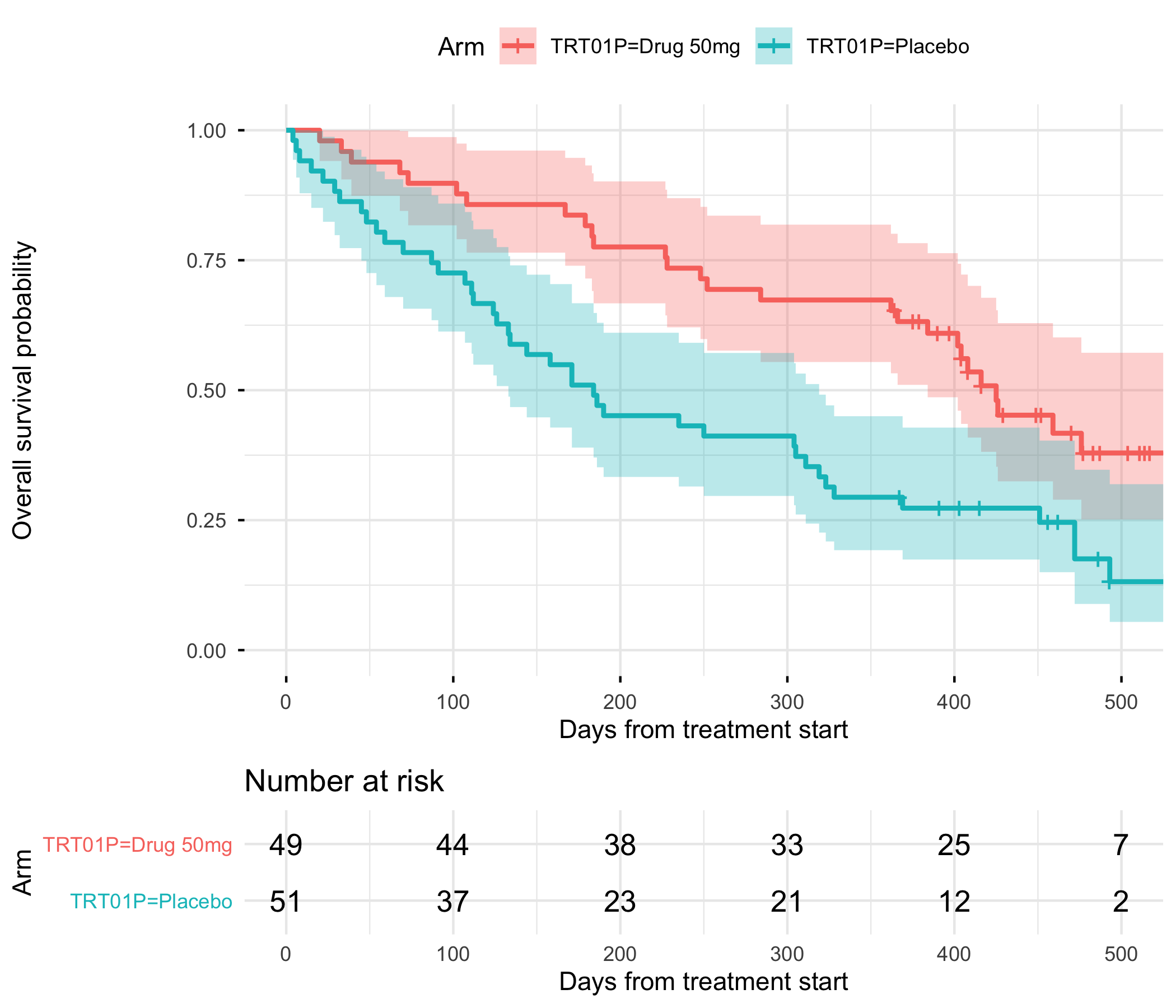
The progression of row granularity across the pipeline is the concept to retain: dm is one row per subject, ex is one row per dose, ds is one row per disposition event, adsl returns to one row per subject, and adtte is one row per subject per parameter. Tracking this at every join is how you avoid silently duplicating subjects; the stopifnot() calls above are the doctrinal minimum.
25.9 The submission package
A complete submission to the FDA is not only SDTM and ADaM datasets. It includes several supporting artifacts:
- Define-XML: machine-readable metadata describing every variable in every dataset, with controlled terminology references, derivations, and provenance. Reviewers ingest it to navigate the submission.
- Annotated CRF (aCRF): the blank CRF with SDTM variable names annotated on each field. It is the bridge from what was collected to what was submitted.
- Study Data Reviewer’s Guide (SDRG) and Analysis Data Reviewer’s Guide (ADRG): narrative PDFs that explain conformance decisions, known issues, and analysis choices.
- Statistical Analysis Plan (SAP): pre-specifies every analysis that appears in the CSR, including populations, estimands, and sensitivity analyses.
You will not usually author Define-XML by hand. Tools such as pinnacle21 and the open-source pharmaverse packages generate it from ADaM specifications.
25.10 The pharmaverse
Until the late 2010s, most ADaM work in industry was done in SAS. Since approximately 2020, a coordinated open-source initiative called the pharmaverse has produced R packages that implement ADaM derivations with validation intended for regulatory use. The principal packages include:
-
admiral(Mancini et al., 2026): modular ADaM derivations. The reference implementation forADSL,ADAE,ADLB,ADTTE, and others. -
metacoreandmetatools: read and validate ADaM specifications. -
xportr: export to SAS transport (XPT) format, which the FDA still requires. -
pharmaverseadam: reference ADaM datasets for teaching and testing.
At a sponsor or CRO that has adopted R, expect to encounter these packages in production pipelines. They are a more useful thing to learn than any proprietary alternative.
25.11 Principle in use
Three habits carry a submission through review:
- Specs before code. Write the ADaM specification first; implement against it. The spec is the contract; the code is the implementation.
-
Verify the censoring convention at the boundary.
CNSR = 1means censored; invert once when crossing into R’ssurvival::Surv(). - Use population flags deliberately. ITT, safety, efficacy, each is a substantive choice the SAP pre-specifies. Match analysis filter to spec.
With AI assistance
TipPrompts to try
- Paste an SDTM domain (even a synthetic one) and ask the LLM to describe its shape, its role, and its relationship to other domains. Check whether the model correctly identifies the granularity (one row per what).
- Give the LLM an
ADSLspecification and ask it to generate anadmiral-style derivation. Compare its output to theadmiralreference implementation. Does it use the correct helper functions, or does it reinvent them? - Ask the LLM to write a reviewer-facing explanation of the
CNSRconvention. Evaluate whether the explanation would be accepted at face value by a new statistician, or whether it contains subtle errors about which value means what.
25.12 Exercises
Extend the
ADTTEin the worked example to include a second parameter, progression-free survival (PFS), stacked as additional rows. Add a synthetic progression event to theDSdomain to support it. Verify thatnrow(adtte) == 2 * n.Build a minimal
ADAE(OCCDS structure) from a fabricatedAESDTM domain. IncludeAEDECOD,AESER,AESEV, and a treatment-emergent flagTRTEMFLderived from whetherAESTDTC >= TRTSDT. Beyond this book’s dependencies. No answer key; these need packages the book does not ship, or a document you write.Install
admiralandpharmaverseadamfrom CRAN. Loadpharmaverseadam::adsland compare its column list to theADSLbuilt in this chapter. Which variables are missing from our simplified version, and which of them would matter for a real oncology analysis?Write an ADaM specification table (in Quarto) for the
ADTTEbuilt above: variable name, label, type, source, and derivation. Render it to PDF.
25.13 Further reading
- CDISC Foundational Standards at
cdisc.org/standards/foundational, the authoritative reference for SDTM and ADaM themselves. -
(Mancini et al., 2026), the
admiralpackage, the CRAN implementation of the ADaM derivations. - (US Food and Drug Administration, 2024), the FDA Study Data Technical Conformance Guide, which states what a submission must contain.
- (International Council for Harmonisation, 2019), for the estimand framework that determines which population flag an analysis should use.
25.14 Prerequisites answers
- SDTM (Study Data Tabulation Model) holds the regulatory view of the raw, collected clinical data, organized into domains such as
DM,AE,LB, andEX. ADaM (Analysis Data Model) holds analysis-ready datasets derived from SDTM. A biostatistician typically builds ADaM; SDTM is built by data management or clinical programmers. -
CNSR = 1indicates a censored observation.CNSR = 0indicates the event of interest. This convention is the inverse ofsurvival::Surv(), which usesevent = 1. -
ADSLis the subject-level anchor dataset. It contains exactly one row per subject, with treatment assignment, demographics, baseline covariates, key dates, and population flags. Every other ADaM dataset (ADLB,ADTTE,ADAE, and so on) joins back toADSLbyUSUBJIDand inherits treatment and population flags from it.