20 Plotting with ggplot2 and purrr
A figure can mislead without printing a single false number. Suppose we draw discharge N-terminal pro-B-type natriuretic peptide (NT-proBNP) for the HF-HOME patients as one bar of means per ejection-fraction stratum, with standard-error whiskers. The figure then says two things: the reduced-ejection-fraction group is higher, and the difference is precise. Both are true of the means. The same values drawn as points show a spread of nearly three orders of magnitude. They also show a mean pulled well above the typical patient by a long right tail, and two groups that overlap almost entirely. The bar chart passed every check its code could make. The problem is in what it lets the reader see. This chapter is about the judgments ggplot2 cannot make for you. It is built around the figure a biostatistician is asked for most often, the trajectory of a repeated measure by treatment arm.
The greatest value of a picture is when it forces us to notice what we never expected to see.
John W. Tukey, Exploratory Data Analysis (1977)
NoteIn this chapter
Reading time. About 30 minutes.
You’ll need. Chapter 15 for long and wide shapes, and Chapter 18 for the joins that assemble the plotting data. The code uses:
You’ll be able to.
- Replace a bar of means with a display of the distribution and its summary, and name what each element encodes.
- Build a longitudinal trajectory figure by arm that shows individual patients, a summary with its uncertainty, and the number measured at each visit.
- Compose panels with facets or
patchwork, and generate one plot per group withpurrr. - Export a themed figure at a journal’s size and format, and audit it against a six-item figure checklist.
Outline.
NoteSkip ahead?
If these answers come quickly, skip to the next chapter. The answers are in Section 20.11.
- How do you produce one plot per level of a categorical variable, returning the results as a named list of
ggplotobjects? - What does
patchwork::wrap_plots()provide thatfacet_wrap()does not? - Why might you save a figure as PDF rather than PNG for a journal submission, and when would you choose PNG instead?
20.1 Show the distribution, not a summary of it
ggplot2 will draw whatever you specify, and the grammar that specifies it is taught well elsewhere.1 Whether the figure communicates or misleads is not something the package can check. The setup chunk below reads the running study and assembles one row per patient visit with an NT-proBNP result. It also sets the house theme and arm colors that every figure in the chapter uses (Section 20.4 explains both).
1 R for Data Science (Wickham et al., 2023, chs. 1, 9, and 11) covers aesthetics, geoms, scales, and labels. For Python, plotnine reproduces the ggplot2 grammar almost verbatim; the judgments in this chapter do not change with the language.
library(tidyverse)
library(patchwork)
arm_colors <- c("Usual care" = "#E69F00", "Home health" = "#0072B2")
scale_color_arm <- function(...) {
scale_color_manual(values = arm_colors, ...)
}
theme_hfhome <- function(base_size = 11) {
theme_minimal(base_size = base_size) +
theme(
panel.grid.minor = element_blank(),
plot.title = element_text(face = "bold"),
legend.position = "bottom"
)
}
theme_set(theme_hfhome())
hf_dir <- file.path("..", "data", "raw_data", "hfhome")
read_hf <- function(file) {
read_csv(file.path(hf_dir, file),
col_types = cols(patient_id = col_character()),
show_col_types = FALSE)
}
randomization <- read_hf("randomization.csv") |>
mutate(
arm = factor(arm, levels = c("Usual care", "Home health")),
ef_stratum = factor(ef_stratum,
levels = c("Reduced EF", "Preserved EF"))
)
visits <- read_hf("visits.csv")
bnp <- read_hf("labs.csv") |>
filter(test_code == "NTPROBNP") |>
distinct() |>
inner_join(visits, by = c("patient_id", "visit_id"),
relationship = "one-to-one") |>
inner_join(randomization, by = "patient_id",
relationship = "many-to-one") |>
mutate(visit = factor(visit_type,
levels = c("discharge", "clinic_day30"),
labels = c("Discharge", "Day 30")))
bnp_discharge <- bnp |> filter(visit == "Discharge")
stopifnot(nrow(bnp_discharge) == nrow(randomization))The distinct() removes the exact duplicate result that Chapter 15 found, and the two relationship = declarations are the join checklist of Chapter 18. The orphan lab patient has no visit row, so the first inner join drops it.
20.1.1 Before and after
bnp_means <- bnp_discharge |>
  summarize(mean = mean(value), se = sd(value) / sqrt(n()),
            .by = ef_stratum)

p_before <- ggplot(bnp_means, aes(ef_stratum, mean)) +
  geom_col(width = 0.6, fill = "grey65") +
  geom_errorbar(aes(ymin = mean - se, ymax = mean + se),
                width = 0.2) +
  labs(x = NULL, y = "NT-proBNP (pg/mL)", title = "Before")

p_after <- ggplot(bnp_discharge, aes(ef_stratum, value)) +
  geom_point(position = position_jitter(width = 0.25, height = 0,
                                        seed = 1),
             alpha = 0.15, size = 0.6) +
  stat_summary(fun = median,
               fun.min = \(x) quantile(x, 0.25),
               fun.max = \(x) quantile(x, 0.75),
               geom = "pointrange", color = "black") +
  scale_y_log10(labels = scales::label_comma()) +
  labs(x = NULL, y = "NT-proBNP (pg/mL, log scale)", title = "After")

p_before + p_after + plot_annotation(tag_levels = "A")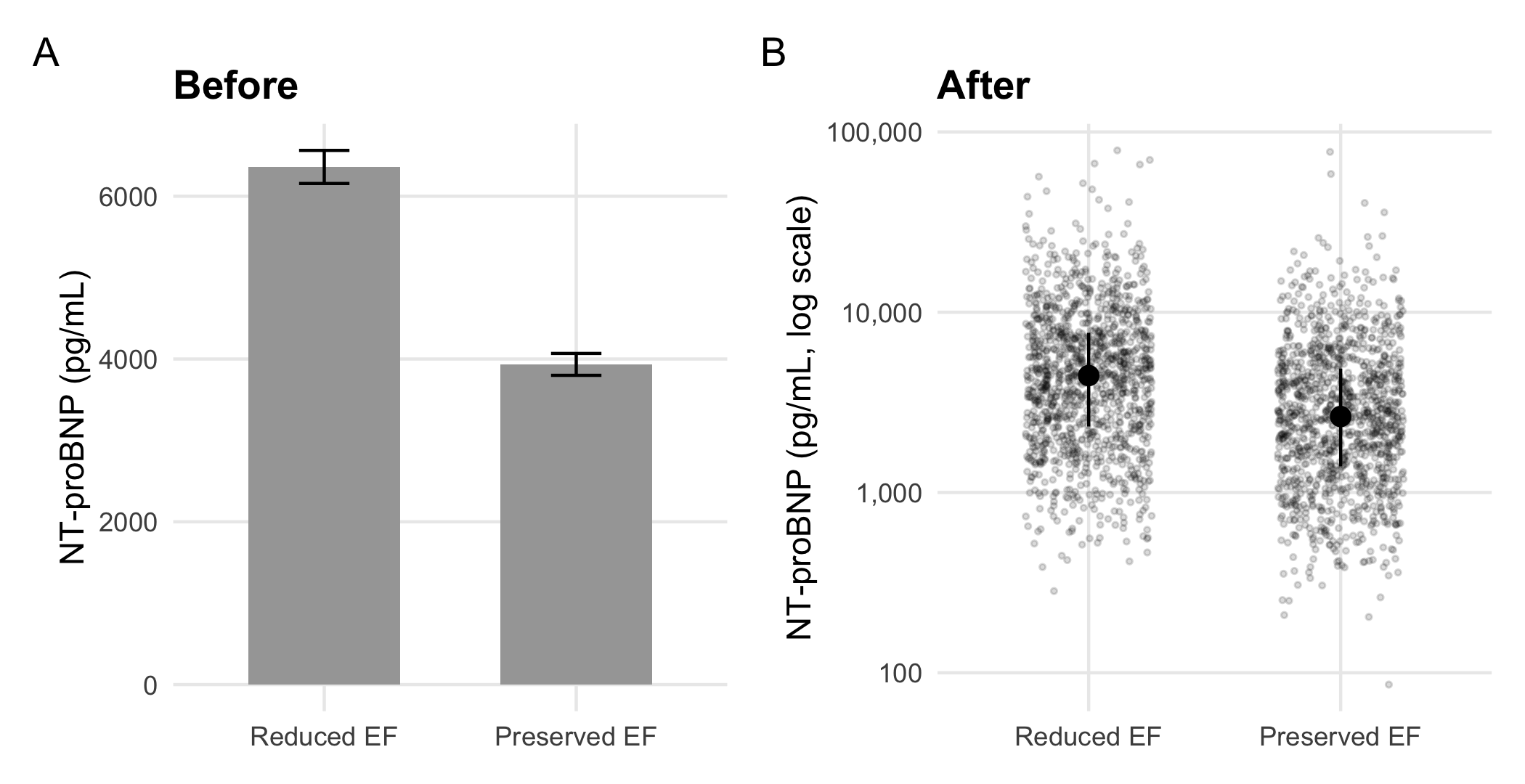
Panel A reports two numbers per group. The reduced-EF bar is a mean of 6,360 pg/mL; the median reduced-EF patient is at 4,453, and the values run from 284 to 79,020. None of that is visible in a bar. Its whiskers are standard errors. These shrink with the sample size and say nothing about how much patients vary. Most of the bar’s ink is a rectangle whose height is measured from a zero that no patient is near. Harrell’s chapter on descriptive graphics (Harrell, 2025, ch. 4) and Weissgerber and colleagues (Weissgerber et al., 2015) make the case at length. That is, plot the data, with the summary overlaid rather than substituted for it.
Three judgments produced panel B, and each recurs in every figure in this chapter:
- State the claim. ‘The strata differ’ is a claim about two distributions, so the figure has to show distributions.
- Name the channel the reader decodes. A bar encodes length from zero; a point encodes position on a scale. A log scale is the honest position scale for a laboratory value whose spread grows with its level.
- Match the display to the density. With about 1,200 points per group, transparency keeps the cloud readable; with ten thousand, a boxplot or violin shows the shape where points would merge into ink.
WarningEthics
The channel a reader decodes is also the channel a figure can distort. A bar whose axis starts above zero exaggerates a difference by the ratio of the visible lengths. An area or bubble that scales a quantity by its radius rather than its area inflates it by a square. Neither is an error R will report. Section 32.5 treats both as misrepresentation, which is how a reader who notices will judge them (Chapter 32).
NoteCheck
Question. A collaborator defends panel A: the whiskers show the uncertainty, so nothing is hidden. What do the whiskers show, and what do they not?
Answer. They show the standard error of each mean, the uncertainty about where the group’s average lies. With about 1,200 patients per stratum that uncertainty is small, so the whiskers are short. They do not show how much patients differ from one another, which is what a reader comparing two groups of patients usually wants to know. They also hide the skew that makes the mean a poor description of the typical patient. Panel B shows both the spread (the points) and a robust summary (median and interquartile range).
20.1.2 Exercises
- Draw discharge creatinine by arm as points with the median and interquartile range, and compute the numbers the summary layer shows. Does creatinine need the log scale that NT-proBNP did?
NoteSolution
creatinine <- read_hf("labs.csv") |>
  filter(test_code == "CREAT", str_ends(visit_id, "-01")) |>
  inner_join(randomization, by = "patient_id",
             relationship = "one-to-one")

creatinine |>
  summarize(median = median(value), q1 = quantile(value, 0.25),
            q3 = quantile(value, 0.75), n = n(), .by = arm)
#> # A tibble: 2 × 5
#>   arm         median    q1    q3     n
#>   <fct>        <dbl> <dbl> <dbl> <int>
#> 1 Home health   1.29  1.02  1.63  1216
#> 2 Usual care    1.3   1.02  1.64  1216

ggplot(creatinine, aes(arm, value)) +
  geom_point(position = position_jitter(width = 0.25, height = 0,
                                        seed = 1),
             alpha = 0.15, size = 0.6) +
  stat_summary(fun = median, fun.min = \(x) quantile(x, 0.25),
               fun.max = \(x) quantile(x, 0.75),
               geom = "pointrange") +
  labs(x = NULL, y = "Creatinine at discharge (mg/dL)")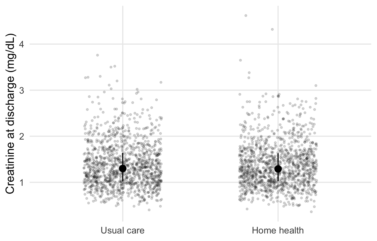
The arms look alike, as randomization intends. Creatinine is right-skewed but spans a far narrower range than NT-proBNP, so a linear scale shows the bulk of the data. A log scale is a choice to make from the spread you see. It is not a default.
20.2 The trajectory figure, layer by layer
A trajectory figure shows a repeated measure over time by arm, with the individual patients visible behind the group summaries. In HF-HOME, NT-proBNP is measured at discharge and at the day-30 clinic visit. The data are already long, one row per patient visit. This is the shape Chapter 15 said a trajectory plot needs: visit is a column, so it can be mapped to the x-axis.
20.2.1 Layer 1: every patient
p_lines <- ggplot(bnp, aes(visit, value)) +
  geom_line(aes(group = patient_id), color = "grey50", alpha = 0.04) +
  scale_y_log10(labels = scales::label_comma()) +
  labs(x = NULL, y = "NT-proBNP (pg/mL, log scale)")
p_lines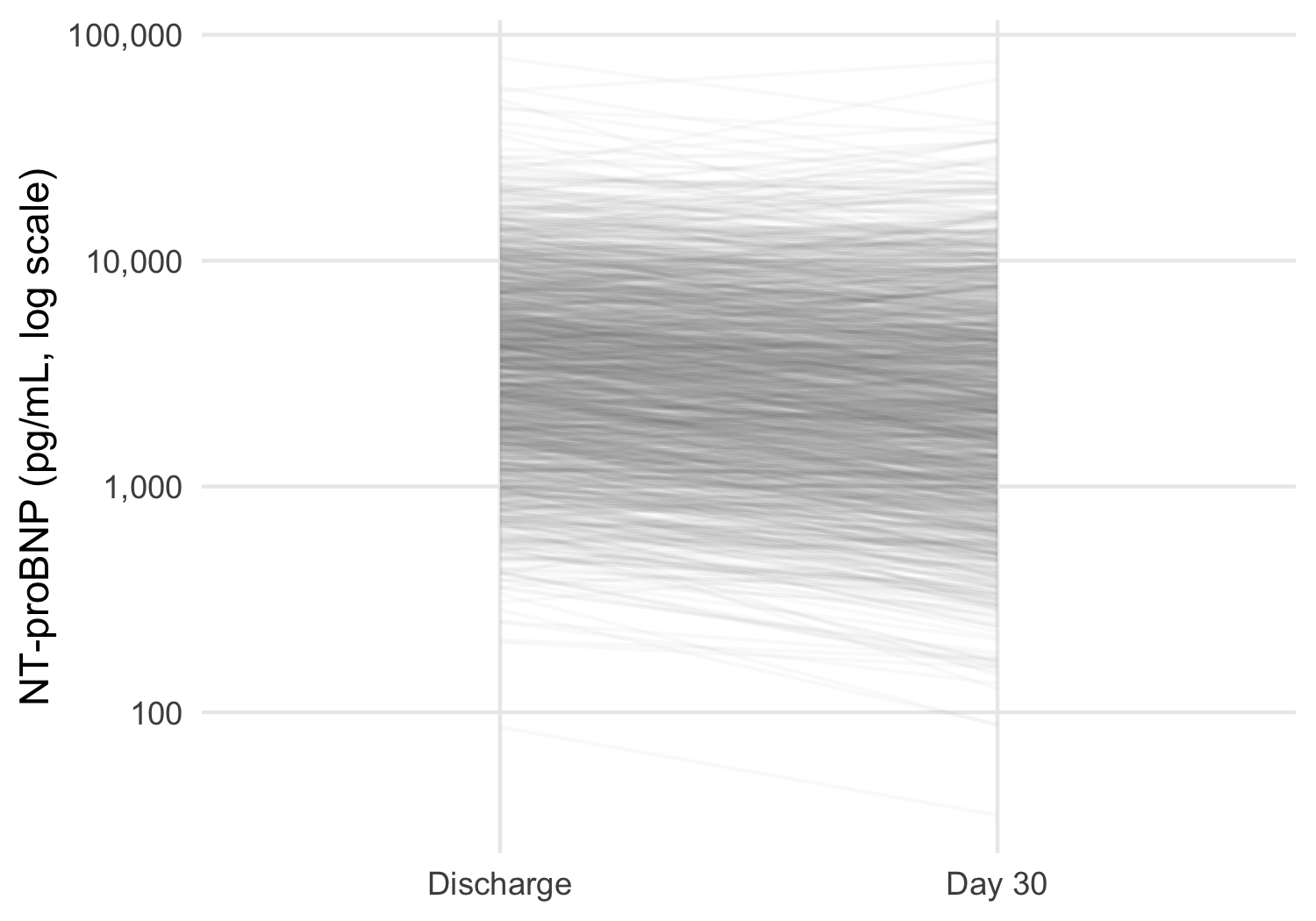
The individual lines show what a plot of means alone would hide: patients move in both directions, and the spread between patients is far larger than any change over 30 days. At this density each line must be nearly transparent. Coloring the lines by arm would only blend two clouds into one indistinct mass, so the arms are left to the next layer.
20.2.2 Layer 2: the summary and its uncertainty
dodge <- position_dodge(width = 0.25)

p_summary <- p_lines +
  stat_summary(aes(color = arm, group = arm), fun = mean,
               geom = "line", position = dodge, linewidth = 0.8) +
  stat_summary(aes(color = arm, group = arm), fun.data = mean_se,
               fun.args = list(mult = 1.96), geom = "pointrange",
               position = dodge) +
  scale_color_arm(name = NULL)
p_summary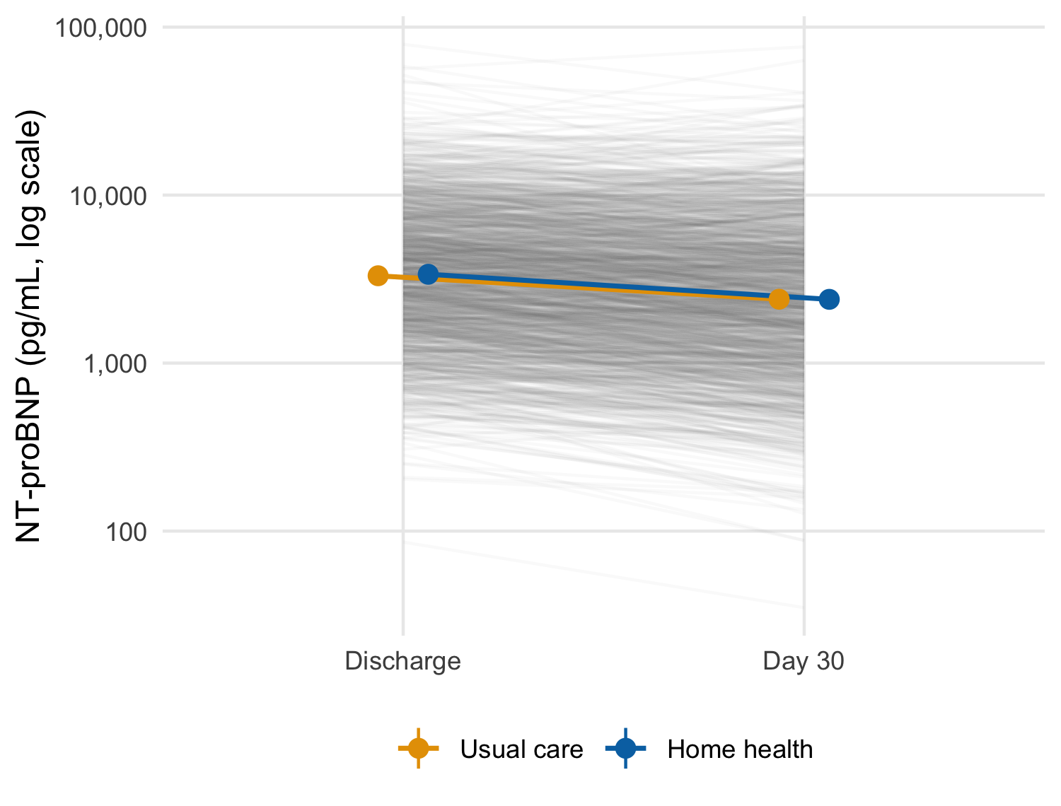
scale_y_log10() transforms the data before the statistics are computed. The mean here is therefore the mean of log values, that is, the geometric mean, with a confidence interval computed on the log scale. For a right-skewed laboratory value that is usually the summary you want, and it matches an analysis of log NT-proBNP.
WarningPitfall
Where the log happens changes the summary. With scale_y_log10() the statistics see log values; with coord_trans(y = "log10") they see raw values, and only the drawing is transformed. The axes look identical, and the plotted means are not.
bnp |>
  summarize(arithmetic = mean(value),
            geometric = exp(mean(log(value))), .by = c(visit, arm))
#> # A tibble: 4 × 4
#>   visit     arm         arithmetic geometric
#>   <fct>     <fct>            <dbl>     <dbl>
#> 1 Discharge Home health      5205.     3379.
#> 2 Day 30    Home health      4073.     2396.
#> 3 Discharge Usual care       5091.     3311.
#> 4 Day 30    Usual care       4162.     2400.
State the summary in the caption, and compute it once with dplyr to confirm that the figure plots what the caption says.
20.2.3 Layer 3: who is still being measured
The day-30 summary is not computed on the same patients as the discharge one.
bnp |> count(visit, arm)
#> # A tibble: 4 × 3
#>   visit     arm             n
#>   <fct>     <fct>       <int>
#> 1 Discharge Usual care   1216
#> 2 Discharge Home health  1216
#> 3 Day 30    Usual care    831
#> 4 Day 30    Home health   817

bnp_discharge |>
  mutate(seen_day_30 = patient_id %in%
           bnp$patient_id[bnp$visit == "Day 30"]) |>
  summarize(n = n(), geometric_mean = exp(mean(log(value))),
            .by = seen_day_30)
#> # A tibble: 2 × 3
#>   seen_day_30     n geometric_mean
#>   <lgl>       <int>          <dbl>
#> 1 TRUE         1648          3304.
#> 2 FALSE         784          3432.
Patients readmitted or dead before day 30 have no clinic visit, so the day-30 point averages over the patients who were well enough to attend. In this draw the patients who missed the visit started only slightly higher, so the selection is small. However, in a trial where the sickest patients drop out, a falling mean line can be produced entirely by who left.
WarningPitfall
A mean trajectory over a shrinking sample shows selection as change. The line between two summaries implies the same patients at both ends. Print the number measured at each visit on the figure, and when attrition is related to the outcome, draw the patients measured at both visits as a sensitivity version.
20.2.4 Exercises
- Compute, without the plot, the geometric mean and 95% confidence interval the summary layer draws for each arm and visit. Then confirm that they match the numbers
ggplot2computed, whichlayer_data()returns. - Redraw the trajectory for the patients measured at both visits only. How many patients per arm remain, and does the picture change?
NoteSolution
by_hand <- bnp |>
  summarize(
    geometric_mean = 10^mean(log10(value)),
    lower = 10^(mean(log10(value)) -
                  1.96 * sd(log10(value)) / sqrt(n())),
    upper = 10^(mean(log10(value)) +
                  1.96 * sd(log10(value)) / sqrt(n())),
    .by = c(arm, visit)
  ) |>
  arrange(arm, visit)
by_hand
#> # A tibble: 4 × 5
#>   arm         visit     geometric_mean lower upper
#>   <fct>       <fct>              <dbl> <dbl> <dbl>
#> 1 Usual care  Discharge          3311. 3141. 3490.
#> 2 Usual care  Day 30             2400. 2231. 2583.
#> 3 Home health Discharge          3379. 3208. 3558.
#> 4 Home health Day 30             2396. 2231. 2574.

from_plot <- layer_data(p_summary, 3) |>
  arrange(group, x)
stopifnot(
  isTRUE(all.equal(by_hand$geometric_mean, 10^from_plot$y)),
  isTRUE(all.equal(by_hand$lower, 10^from_plot$ymin))
)
layer_data() returns what the layer actually drew, on the scale it drew it (log10 here). Comparing it with an independent dplyr computation is the figure’s equivalent of a unit test. It confirms that the caption’s ‘geometric mean and 95% CI’ describes the points.
NoteSolution
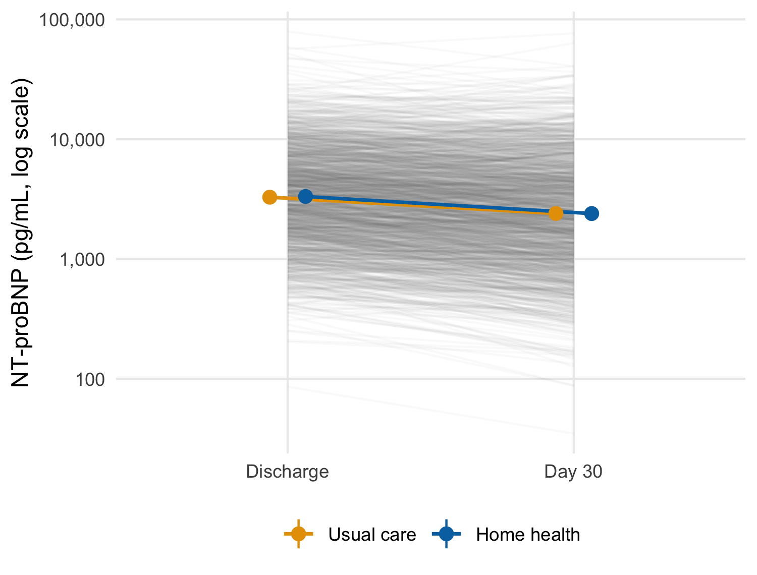
Adding a data frame to a plot with + replaces its data and keeps every layer.2 Here the completers’ trajectory is close to the full version. This is consistent with the small difference at discharge between patients who did and did not attend the day-30 visit. Report the check either way, since a sensitivity version that agrees is still evidence.
2 Versions of ggplot2 before 4.0 needed the %+% operator for this; 4.0 deprecates it in favor of +.
NoteCheck
Question. The two arms’ 95% intervals overlap at day 30. Can you conclude from the figure that home health had no effect on NT-proBNP?
Answer. No. Overlapping intervals for two groups do not establish that the difference between them is zero, or even that it is not significant. The interval for the difference is the quantity that answers the question (Chapter 32 returns to this fallacy). The figure is descriptive. The treatment comparison belongs to the pre-specified analysis in Chapter 26, and the figure should not be read as its substitute.
20.3 Panels: facets, patchwork, and many plots
Two tools put several panels in one figure, and they answer different questions (Table 20.1).
| Tool | Panels are | Use when |
|---|---|---|
facet_wrap(), facet_grid()
|
The same plot, conditioned on a variable | Comparing one display across strata or sites |
patchwork (+, /, wrap_plots()) |
Independent plots, which may differ in everything | Combining different views into one figure |
split() with purrr::imap()
|
Separate figures, one per group | One file per site for a report or a monitoring committee |
20.3.1 Facets: the same plot, by stratum
p_summary + facet_wrap(vars(ef_stratum))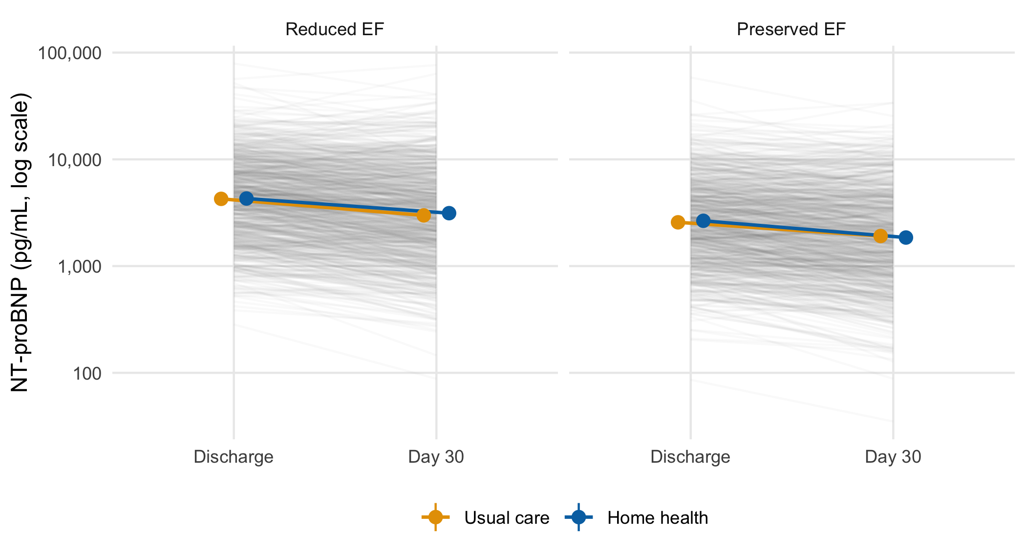
20.3.2 Patchwork: different views in one figure
(p_after + labs(title = NULL)) + p_summary +
  plot_layout(guides = "collect") +
  plot_annotation(tag_levels = "A")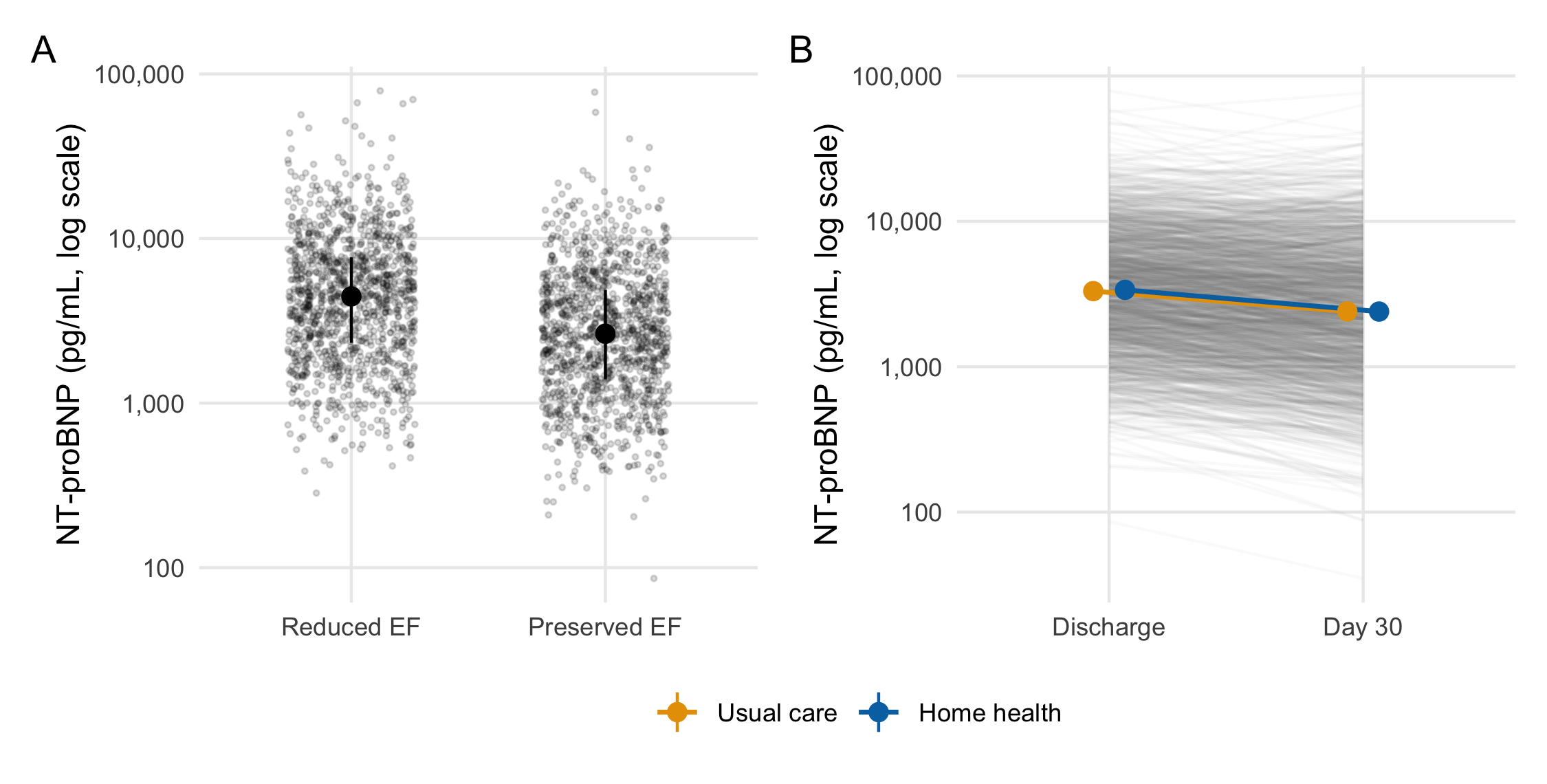
plot_annotation(tag_levels = 'A').
plot_annotation(tag_levels = "A") letters the panels in layout order and keeps the letters correct when panels are added or moved. Letters typed into labs(title = "A. ...") have to be renumbered by hand. plot_layout(guides = "collect") gathers duplicate legends into one.
20.3.3 One plot per group with purrr
split() returns a named list, and imap() passes each element and its name to a function. walk2() then writes the files. This is a side effect, so walk2() returns nothing:
site_plots <- bnp |>
  split(bnp$site) |>
  imap(\(d, site) p_summary + d + labs(title = site))

site_dir <- file.path(tempdir(), "site-figures")
dir.create(site_dir, showWarnings = FALSE)
walk2(site_plots,
      file.path(site_dir, paste0(names(site_plots), ".png")),
      \(p, path) ggsave(path, p, width = 5, height = 3.8, dpi = 150))
list.files(site_dir)
#> [1] "Site A.png" "Site B.png" "Site C.png" "Site D.png" "Site E.png"
NoteCheck
Question. You want the discharge distribution by stratum and the trajectory by arm in one figure. Why does facet_wrap() not do it?
Answer. Facets draw the same plot, with the same geoms and the same mapping, in each panel, conditioned on a variable. These are two different plots, with different x variables and different layers, so they are composed with patchwork. Faceting is the right tool when the second panel is the first one again for a different subset, as in the stratum figure above.
20.3.4 Exercises
- Write
plot_by(data, var), which returns a named list of trajectory plots, one per level of the column named by the stringvar. Apply it tositeand toef_stratum, and report the names of each list.
NoteSolution
data[[var]] takes the column name as a string, which is right when the caller holds the name in a variable (Chapter 15). imap() rather than map() is what gives each plot its group name for the title. split() names the list by level, in factor order for a factor and alphabetical order for a character column.
20.4 Theme, color, and export
20.4.1 Set the theme once, and add it where a plot travels
The setup chunk defined theme_hfhome() and called theme_set(theme_hfhome()) once, at the top of the document, where anyone reading the source sees it before the first plot. That is the right place for it in an analysis script or report. However, it is also invisible state. A plot lifted into a slide deck or a colleague’s session renders with ggplot2’s defaults, with no error. Anything whose pieces travel (a function that returns a plot, a figure prepared for slides) should add the theme explicitly. The worked example’s function does this with + theme_hfhome(). The explicit form also makes opting out possible, for a figure that must follow a journal’s style instead of the house one.
20.4.2 Choose colors that survive color-vision deficiency
About one man in twelve has a red-green color-vision deficiency. The arm colors come from the Okabe-Ito palette (palette.colors(palette = "Okabe-Ito") in base R). They are named by arm level, so a subset or a reordered factor cannot attach the wrong color to an arm. Check a palette by simulating each deficiency and measuring how far apart the colors remain:
color_distance <- function(colors) {
  simulated <- list(
    normal = colors,
    deutan = colorspace::deutan(colors),
    protan = colorspace::protan(colors),
    tritan = colorspace::tritan(colors)
  )
  map_dbl(simulated, \(x) farver::compare_colour(
    farver::decode_colour(x[1]), farver::decode_colour(x[2]),
    from_space = "rgb", method = "cie2000"
  )[1, 1])
}

round(color_distance(arm_colors), 1)
#> normal deutan protan tritan
#>   55.3   62.6   55.5   51.4
round(color_distance(c("#D62728", "#2CA02C")), 1)
#> normal deutan protan tritan
#>   71.8    4.8   24.9   65.3
The numbers are CIEDE2000 color differences, on which a difference of a few units is near the limit of perception. The arm colors stay far apart under every simulation. The familiar red and green pair, on the other hand, becomes nearly indistinguishable under deuteranopia.
20.4.3 Export for the destination
ggsave() picks the format from the file extension. Size the figure at the dimensions it will be printed, in the journal’s units, so that text and line widths come out at the sizes you saw. Table 20.2 summarizes the usual choices. Where they differ, the journal’s author instructions take precedence.
| Destination | Format |
ggsave() settings |
Note |
|---|---|---|---|
| LaTeX or journal production | PDF, vector |
device = cairo_pdf, units = "mm"
|
Embeds fonts, so the PDF renders on systems that lack them |
| Word, slides | PNG, raster |
dpi = 300 at the final size |
Line art is often requested at 600 dpi or more |
| Web | SVG, vector | needs the svglite package |
Stays sharp on zoom |
| Single journal column | any |
width = 85 to 90, units = "mm"
|
Typical; check the journal |
| Full page width | any |
width = 170 to 180, units = "mm"
|
Typical; check the journal |
20.4.4 Exercises
- Save
p_summaryas a PNG one journal column wide (85 mm) and 80 mm high at 300 dpi. Predict its pixel dimensions, then read the file back withpng::readPNG()and check your prediction.
NoteSolution
png_path <- file.path(tempdir(), "trajectory-85mm.png")
ggsave(png_path, p_summary, width = 85, height = 80, units = "mm",
       dpi = 300)

expected <- round(c(height = 80, width = 85) / 25.4 * 300)
actual <- dim(png::readPNG(png_path))[1:2]
expected
#> height  width
#>    945   1004
actual
#> [1]  944 1003
stopifnot(all(abs(actual - expected) <= 1))
Pixels are millimeters divided by 25.4, times the dpi, so 85 mm at 300 dpi is about 1,004 pixels wide. A figure saved large and shrunk by the journal comes out with text too small to read. Saving at the printed size is what keeps the 11-point base font at 11 points.
20.5 Accessible figures
Every figure in this chapter carries a fig-alt string, but the chunks so far have not said what makes one good. A figure can be inaccessible to three overlapping audiences. The first is a reader using a screen reader, who never sees the pixels and depends entirely on the alt text. The second is a reader with a color-vision deficiency, who sees the pixels but not the colors as drawn. The third is a reader with low vision or on a low-quality display, who sees the colors but not a weak contrast between them. Each has a specific, checkable fix.
20.5.1 Alt text describes the claim, not the chart
A screen reader announces the fig-alt text in place of the image. ‘Bar chart’ or ‘a plot of NT-proBNP’ tells that reader a figure exists and nothing else. It names the picture and omits what looking at it would tell a sighted reader. Good alt text states the pattern on which the figure rests its case, in the same terms the caption’s claim uses. It does not require the reader to infer the finding from chart-type vocabulary. Compare the chapter’s own @fig-bar-vs-points. Its alt text names the two panels, the fact that the clouds ‘overlap almost entirely’, and where the medians sit, which is the finding panel B exists to show. It would fail that test if it read only ‘two panels of NT-proBNP by ejection-fraction stratum’. @fig-trajectory‘s alt text goes further and states the direction of the arm summaries (’fall from discharge to day 30 and overlap at both visits’). It does so because that direction is the figure’s point.
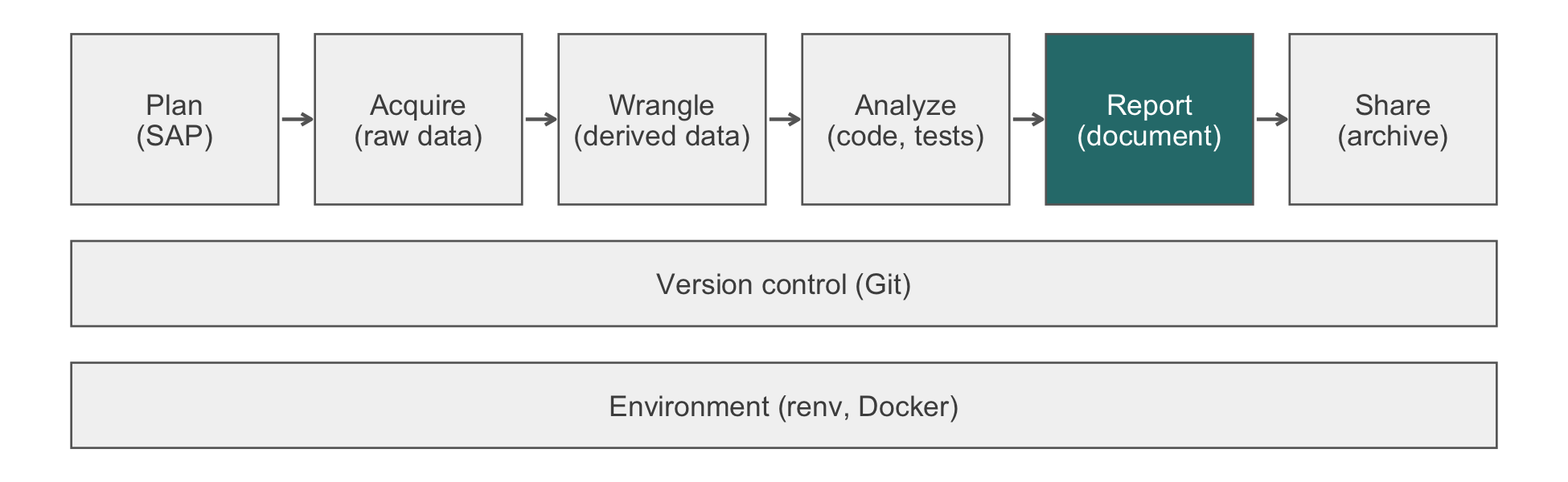
Three practical rules follow. First, state the shape or trend before any decoration (‘two clouds of points overlapping almost entirely’, not ‘a scatter plot with jittered points’). Second, do not merely restate the caption word for word. A sighted reader reads the caption alongside the image, but a screen reader moving past the figure may skip it. The alt text is then the only description some readers get, so it should stand alone. Third, reserve a short or empty alt text for a genuinely decorative figure, one that illustrates rather than reports a result. This chapter’s pipeline diagrams (fig-alt: !expr pipeline_alt('report')) name only the pipeline stage, which is all that figure is for.
20.5.2 Color that survives color-vision deficiency
Section 20.4 already builds the arm palette from Okabe-Ito. It checks the palette under simulated deficiencies with colorspace::deutan() and related functions. That check is the general method, and two further rules apply broadly. First, color should be redundant with position, a label, or a line type whenever the figure’s claim depends on telling groups apart. The trajectory figure’s arms differ in color and in dodge position. A reader who cannot tell orange from blue can still separate them by where the point sits. Second, Okabe-Ito’s eight unordered colors do not suit an ordered or continuous variable. For such a variable, use a perceptually uniform, colorblind-safe sequential palette such as viridis, which is available in ggplot2 without an extra package:
bnp_discharge |>
  left_join(read_hf("demographics.csv") |>
              select(patient_id, age),
            by = "patient_id", relationship = "one-to-one") |>
  ggplot(aes(ef_stratum, value, color = age)) +
  geom_point(position = position_jitter(width = 0.25, height = 0,
                                        seed = 1),
             alpha = 0.5) +
  scale_y_log10() +
  scale_color_viridis_c() +
  labs(x = NULL, y = "NT-proBNP (pg/mL, log scale)")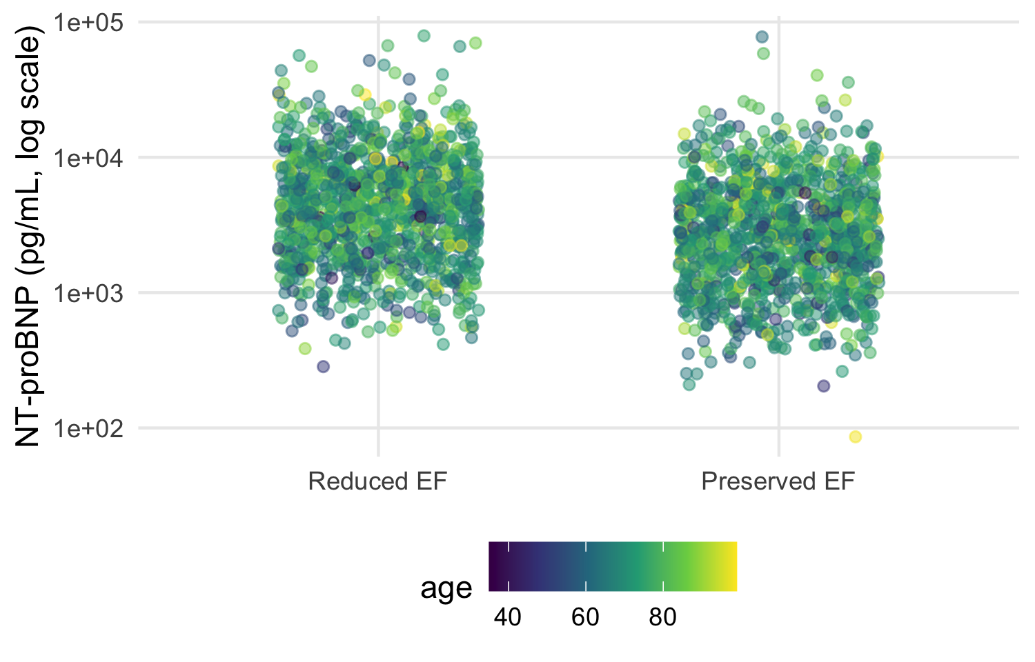
Viridis remains perceptually uniform and distinguishable under every common deficiency simulated above. A rainbow or red-to-green scale does not. Both distort the data’s apparent ordering, and both lose their distinctions under red-green deficiencies.
20.5.3 Contrast: the WCAG practical minimum
The Web Content Accessibility Guidelines set numeric contrast minimums for level AA conformance (World Wide Web Consortium, 2018). Two of them apply to a figure. Text (axis labels, titles) needs a 4.5:1 ratio, and a graphical object or its boundary needs a 3:1 ratio against its background (WCAG 1.4.3 and 1.4.11). The ratio is computed from each color’s relative luminance, not from how different the colors look by eye:
relative_luminance <- function(hex) {
  rgb <- col2rgb(hex) / 255
  rgb <- ifelse(rgb <= 0.03928, rgb / 12.92, ((rgb + 0.055) / 1.055)^2.4)
  0.2126 * rgb[1, ] + 0.7152 * rgb[2, ] + 0.0722 * rgb[3, ]
}
contrast_ratio <- function(color, background) {
  l <- relative_luminance(c(color, background))
  (max(l) + 0.05) / (min(l) + 0.05)
}
round(map_dbl(arm_colors, contrast_ratio, background = "white"), 2)
#>  Usual care Home health
#>        2.25        5.19
Both arm colors clear 3:1 against the white panel background theme_hfhome() draws, so the point and line marks meet the graphical-object minimum. Axis text, drawn in near-black by theme_minimal(), clears the stricter 4.5:1 text minimum by a wide margin. A pale color that passes a by-eye check often fails this ratio against a white background. For this reason the house palette is checked by computation rather than by looking at it on one screen.
NoteCheck
Question. A colleague proposes "grey80" for a reference line that must stay visible against the white panel background. Is that safe for a figure meant to meet WCAG AA?
Answer. Compute it. contrast_ratio("grey80", "white") is about 1.3, far below the 3:1 minimum for a graphical object. The line would be close to invisible for a low-vision reader, even though it looks faint but present on a well-calibrated screen. A mid-gray closer to "grey40" or a line pattern (dashed, not merely lighter) clears the minimum. It also survives printing in black and white.
20.5.4 Exercises
- Compute the contrast ratio of
"grey65", the fill used for panel A’s bars in@fig-bar-vs-points, against white. Does the bar chart that this chapter replaces meet the graphical-object minimum, and does passing that check answer whether the bar chart is a good figure?
NoteSolution
contrast_ratio("grey65", "white")
#> [1] 2.434354
The ratio is a little above 3:1, so the bars themselves are legible against the white background. However, passing the contrast check says nothing about the chapter’s earlier objection to panel A. A legible bar can still misrepresent the data it summarizes.
20.6 Worked example: the trajectory figure, end to end
The function below assembles the chapter’s layers into the figure a report would carry. It takes the long data and returns a plot, so the same code draws the full trial, a site, or a sensitivity subset. It adds the theme explicitly because the plot is meant to be reused elsewhere.
plot_trajectory <- function(data) {
  n_visit <- data |>
    count(visit, arm) |>
    pivot_wider(names_from = arm, values_from = n)
  visit_labels <- set_names(
    paste0(n_visit$visit, "\n",
           scales::comma(n_visit$`Usual care`), " / ",
           scales::comma(n_visit$`Home health`)),
    n_visit$visit
  )
  dodge <- position_dodge(width = 0.25)

  ggplot(data, aes(visit, value)) +
    geom_line(aes(group = patient_id), color = "grey50",
              alpha = 0.04) +
    stat_summary(aes(color = arm, group = arm), fun = mean,
                 geom = "line", position = dodge, linewidth = 0.8) +
    stat_summary(aes(color = arm, group = arm), fun.data = mean_se,
                 fun.args = list(mult = 1.96), geom = "pointrange",
                 position = dodge) +
    scale_y_log10(labels = scales::label_comma()) +
    scale_x_discrete(labels = visit_labels) +
    scale_color_arm(name = NULL) +
    labs(x = "Visit (patients measured: usual care / home health)",
         y = "NT-proBNP (pg/mL, log scale)") +
    theme_hfhome()
}

p_trajectory <- plot_trajectory(bnp)
p_trajectory

fig_dir <- file.path(tempdir(), "figures")
dir.create(fig_dir, showWarnings = FALSE)
ggsave(file.path(fig_dir, "bnp-trajectory.pdf"), p_trajectory,
       width = 170, height = 120, units = "mm", device = cairo_pdf)
ggsave(file.path(fig_dir, "bnp-trajectory.png"), p_trajectory,
       width = 170, height = 120, units = "mm", dpi = 300)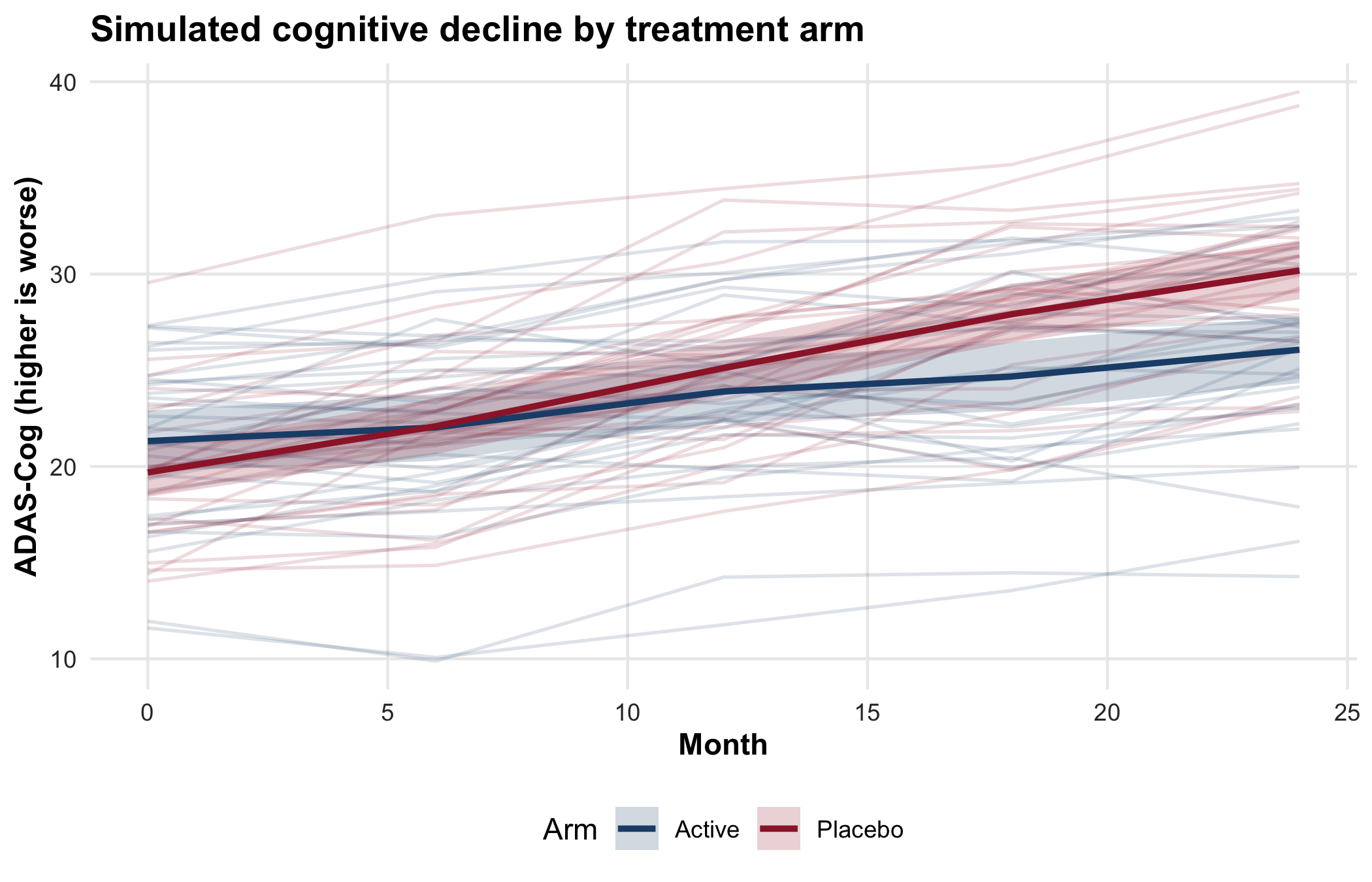
The figure answers one descriptive question: how NT-proBNP moved over 30 days in each arm, and how much patients varied around that movement. It does not claim a treatment effect, and its intervals are not a test. The comparison between arms belongs to the pre-specified analysis. The script writes the files to a temporary directory so that rendering the book leaves the repository unchanged. In a compendium, fig_dir is the project’s figures/ directory, and the files are rebuilt whenever the data change.
TipVerification
Confirm that the counts printed under the axis are the counts in the data, and that both files were written.
axis_labels <- p_trajectory$scales$get_scales("x")$labels
counted <- bnp |> count(visit, arm)
label_matches <- map2_lgl(
  as.character(counted$visit), counted$n,
  \(v, n) str_detect(axis_labels[[v]], scales::comma(n))
)
stopifnot(
  all(label_matches),
  all(file.exists(file.path(fig_dir, c("bnp-trajectory.pdf",
                                       "bnp-trajectory.png"))))
)
axis_labels
#>                  Discharge                     Day 30
#> "Discharge\n1,216 / 1,216"        "Day 30\n831 / 817"
The labels were computed inside the function, so the check compares them with an independent count(). Each arm’s count at each visit must appear in that visit’s label. Discharge shows every randomized patient in each arm, and day 30 fewer.
Every figure in a report should pass the six checks in Table 20.3, which collect this chapter’s judgments.
| Check | Question to ask | In the trajectory figure |
|---|---|---|
| Claim | What single statement is the figure for? | How NT-proBNP changed by arm over 30 days, and how much patients varied |
| Channel | What is the reader’s eye measuring? | Position on a log scale; no bars, areas, or truncated baselines |
| Distribution | Is the variation visible, not only a summary? | Every patient’s line behind the summaries |
| Uncertainty | Does every estimate carry its interval, with the summary named? | Geometric means with 95% intervals; the caption says so; numbers measured per visit |
| Theme | Does it match the other figures, with a palette safe for color-vision deficiency? |
theme_hfhome() added explicitly; Okabe-Ito colors named by arm |
| Export | Is it saved by code, at the printed size, in the destination’s format? |
ggsave() at 170 mm, PDF with cairo_pdf and PNG at 300 dpi |
20.6.1 One way to automate this: zzlongplot
The in-house zzlongplot package (Appendix C, version 0.6.0) draws this kind of figure from a formula. It shows the number measured at each point by default and includes a change-from-baseline panel. The hand-written stat_summary() version above needs extra code to add either. The package is optional. The ggplot2 function above is the portable approach, and everything in this chapter works without zzlongplot. The package is installed from GitHub only (github.com/rgt47/zzlongplot) and is maintained by one person. The block below is display-only because the package is not in the book’s lockfile.
Before it was presented here, zzlongplot was rerun against the HF-HOME discharge and day-30 NT-proBNP values (log10 scale) by arm and visit. Its output was compared with the stat_summary() figure above, which uses mean_se with mult = 1.96. The two agreed on the mean and the 95% interval bounds to three decimal places in all four arm-by-visit cells. This was checked once on 2026-10-10 and again on 2026-10-11. With over a thousand patients per arm, the package’s t interval and the figure’s normal-approximation interval differ by far less than that. The package’s 312-test suite checks the interval arithmetic itself: the t interval, the standard error, and the coverage. One caveat is a property of the data, not of the package. As Section 20.2 shows for the hand-written figure, zzlongplot’s day-30 means reflect only the patients who attended that visit. A falling day-30 mean can therefore reflect who stayed in the trial rather than a change in anyone’s value. Its runnable example takes about 21 seconds, longer than the figures in this chapter, because it fits each panel’s interval itself rather than reusing one already computed.
Use it when it saves you code on a standard longitudinal design, and once the comparison above has been run for the data at hand (as Exercise 2 checks this chapter’s hand-written figure). Write your own when the encoding, the layout, or the summary is not one the package supports.
ImportantLLM prompt
Use a model to draft a figure, with the checklist as the acceptance criteria.
Context.
bnpis a long data frame with one row per patient visit:patient_id(character),visit(factor: Discharge, Day 30),arm(factor: Usual care, Home health), andvalue(NT-proBNP, pg/mL, right-skewed). Attendance falls at day 30.Constraints. Use
ggplot2only. Draw individual patients as faint lines; summarize each arm withstat_summary()on ascale_y_log10()axis; show the number measured per arm at each visit; use the colors inarm_colors. No bars, nogeom_smooth(), nocoord_trans(). Letter any panels withplot_annotation(tag_levels = "A").Criteria. State in the caption which summary and interval are drawn. Return a function of the data, not a plot of a global object. List your assumptions before writing code.
Failure mode. Models default to a bar of means with error bars, or to arithmetic means with a log axis added afterward, and they type panel letters into titles. Check. Walk Table 20.3 row by row, and compare layer_data() with a dplyr summary as in Exercise 2. The prompt sends variable names and types, not data (Section 12.3).
NoteCheck
Question. A reviewer asks for the trajectory figure ‘with the p-value on it’. What do you say?
Answer. The figure is descriptive. Its job is to show the data, their variation, and the attrition. The treatment comparison is the pre-specified analysis, reported with its estimate and interval in the results. A p-value placed on a figure of per-visit summaries invites the reader to treat overlapping per-arm intervals as the test. Offer the estimate and interval of the pre-specified contrast in the text or a table, and keep the figure for what it shows.
20.7 Rules of thumb
- Habit 8: a plausible figure can be a wrong one. A bar of means and a mean line over a shrinking sample both look right; show the distribution and the number measured.
-
Habit 10: every number is computed, including the ones in a figure. Build figures with functions, save them with
ggsave(), and checklayer_data()against an independent summary. - Habit 11: lead with the answer. One claim per figure, named in the caption, and no more claimed than the design supports.
20.8 Cumulative practice
- Cumulative (uses Chapter 18 and Chapter 15). Draw the creatinine trajectory across all three visit types (discharge, home health, day 30) by arm. Assemble the data with declared join relationships, show the number measured per arm at each visit type, and explain what the middle time point compares.
- On your own work (no key). Find a bar-of-means figure in a paper you have read recently, redraw it from its data or a simulation of similar shape as points with summaries, and audit both versions against Table 20.3.
NoteSolution to exercise 6
creatinine_long <- read_hf("labs.csv") |>
  filter(test_code == "CREAT") |>
  inner_join(visits, by = c("patient_id", "visit_id"),
             relationship = "one-to-one") |>
  inner_join(randomization, by = "patient_id",
             relationship = "many-to-one") |>
  mutate(visit = factor(visit_type,
                        levels = c("discharge", "home_health",
                                   "clinic_day30"),
                        labels = c("Discharge", "Home health",
                                   "Day 30")))

creatinine_long |> count(visit, arm)
#> # A tibble: 6 × 3
#>   visit       arm             n
#>   <fct>       <fct>       <int>
#> 1 Discharge   Usual care   1216
#> 2 Discharge   Home health  1216
#> 3 Home health Usual care    132
#> 4 Home health Home health  2105
#> 5 Day 30      Usual care    831
#> 6 Day 30      Home health   817

plot_trajectory(creatinine_long) +
  scale_y_continuous(name = "Creatinine (mg/dL)")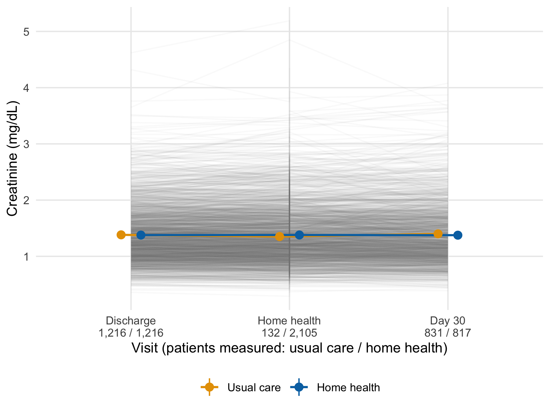
The function needed no change, which is the benefit of writing it as a function of the data. Only the y scale is replaced, because creatinine does not need the log axis. The middle time point is not a comparison of the arms. Home-health visits happen mostly in the home-health arm, so the few usual-care values there come from patients who received home health outside the protocol. A patient with several home-health visits also contributes several values, which the vertical strokes at the middle visit show. The count labels are what make this visible. Without them the middle points read as a fair comparison.
20.9 Cheat sheet
| Task | Code | Guards against |
|---|---|---|
| Show points and a robust summary |
geom_point(position = position_jitter(seed = 1)) + stat_summary(fun = median, ...)
|
A bar of means hiding the distribution |
| Log axis, statistics on log values | scale_y_log10() |
Arithmetic means of skewed values |
| Individual trajectories | geom_line(aes(group = patient_id), alpha = 0.04) |
Means that hide heterogeneity |
| Mean and 95% CI per group | stat_summary(fun.data = mean_se, fun.args = list(mult = 1.96)) |
Estimates without intervals |
| Separate overlapping groups | position_dodge(width = 0.25) |
Arms overprinting each other |
| Same plot by stratum | facet_wrap(vars(ef_stratum)) |
One panel per subset built by hand |
| Compose different plots | p1 + p2 + plot_layout(guides = "collect") |
Duplicate legends |
| Letter panels | plot_annotation(tag_levels = "A") |
Hand-typed letters out of order |
| One plot per group | split(df, df$site) \|> imap(...) |
Copy-pasted plotting code |
| Write files in a loop | walk2(plots, paths, \(p, f) ggsave(f, p)) |
A list of NULL returns |
| Replace a plot’s data | p + new_data |
Rebuilding layers for a subset |
| Check what was drawn | layer_data(p, i) |
A caption that does not match the plot |
| House theme |
theme_set(theme_hfhome()) once; + theme_hfhome() on traveling plots |
Default styling in another document |
| Named palette | scale_color_manual(values = c("Usual care" = ...)) |
Colors attached to the wrong group |
| Export at printed size | ggsave(f, p, width = 85, units = "mm", dpi = 300) |
Unreadable text after scaling |
20.10 Further reading
-
(Wilke, 2019), Fundamentals of Data Visualization, the principles behind the checklist, at
clauswilke.com/dataviz. - (Weissgerber et al., 2015), on why bar graphs of continuous data mislead and what to draw instead.
-
(Wickham et al., 2023) Chapters 1, 9, and 11, the
ggplot2grammar, layers, and labeling, for the generic tour this chapter omits. - (World Wide Web Consortium, 2018), the Web Content Accessibility Guidelines, for the full contrast and text-alternative requirements that Section 20.5 summarizes to a practical minimum.
20.11 Prerequisites answers
-
split(data, data$group) |> map(\(d) ggplot(d, aes(x, y)) + geom_point())returns a named list of plots, one per group, becausesplit()names its output by level;imap()in place ofmap()also passes each name, for titles or file names. Adplyralternative isdata |> group_by(group) |> group_map(\(d, k) ggplot(d, aes(x, y)) + geom_point()), butgroup_map()returns an unnamed list, so the names must be added afterward, for example withset_names(group_keys(grouped)$group), wheregroupedis the grouped data. -
facet_wrap()splits a single plot into panels by a variable; every panel shares the same mapping, geoms, and scales.patchwork::wrap_plots()composes distinct plots that may differ in every respect (geoms, data, scales). Use facets for small multiples of one plot, andpatchworkfor a figure made of different views. - PDF is a vector format: it scales cleanly, embeds fonts, and is what journal production systems prefer for typeset output. PNG is raster, appropriate for Word documents, slides, and web pages where vector support is limited. Save PDF for LaTeX submissions and PNG at 300 dpi, at the printed size, for Word.