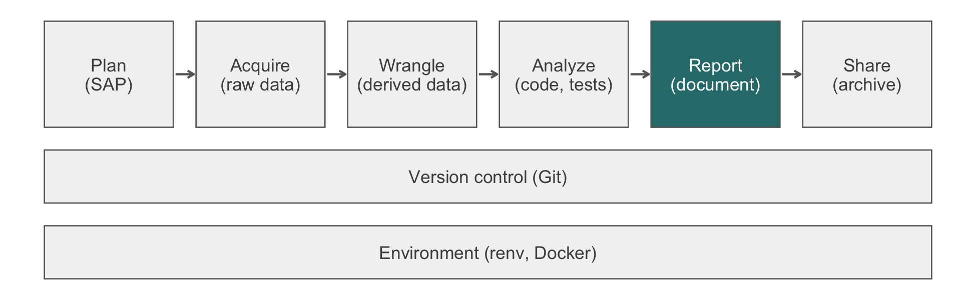
33 Communicating a Finished Analysis
The week after database lock, Dr. X sends a one-line email: ‘So did it work?’ For HF-HOME the honest answer is that the trial cannot tell. Its interval runs from a small harm to a benefit larger than the one it was designed to detect. Two easy replies are available, and both are wrong in ways that are easy to miss. The first is ‘no, it was not significant’, which a reader takes to mean ‘home health does not work’. The second is ‘yes, readmissions fell by two and a half points’, which a reader takes as a finding. Neither contains a false number. This chapter is about the reply that is right. It is also about the three documents in which a statistician is judged on it: the memo, the talk, and the response to reviewers.
The great enemy of communication, we find, is the illusion of it.
William H. Whyte, ‘Is Anybody Listening?’, Fortune (1950)
NoteIn this chapter
Reading time. About 35 minutes.
You’ll need. Chapter 3 for the three registers of a claim, Chapter 26 for the HF-HOME statistical analysis plan (SAP), and Section 21.6 for the tipping-point analysis. The code reads the running study’s files and uses:
You’ll be able to.
- Classify an interval as a precise null, inconclusive, benefit, or harm against zero and the minimum clinically important difference (MCID), and state what it rules out.
- Write a one-page, answer-first memo whose every number is computed, and name the parts it must contain.
- Report a two-dimensional tipping-point analysis as the set of departures from the primary assumption that would change the conclusion.
- Draft a point-by-point response to reviewers that concedes, performs, or declines each request on technical grounds.
Outline.
NoteSkip ahead?
If these answers come quickly, skip to the next chapter. The answers are in Section 33.14.
- Why is the order in which you conducted an analysis almost never the right order in which to present it?
- Your primary analysis found no effect. What, precisely, is the difference between reporting that as ‘no evidence of an effect’ and as ‘evidence of no effect’, and which one are you usually entitled to?
- A reviewer asks you to re-run the primary analysis with a different exclusion criterion. What in your compendium determines whether that costs you an hour or a week?
33.1 Argument, not chronology
An analysis is a chronology: you obtained the data, cleaned it, described it, modeled it, checked the model, and arrived at an estimate. That order is right for doing the work, for the compendium, and for the methods section. It is wrong for almost every act of communication. It withholds what the audience came for until the end. It also asks them to hold six irrelevant facts in memory on the promise that they will matter later.
Presenting an analysis is argument: here is the claim, here is the evidence, here is what would have changed my mind. The three genres in this chapter are three audiences for that argument. The talk gets the least evidence and the most argument. The response to reviewers gets the most evidence and the least latitude. Everything in them is a matter of judgment, and no tool does it for you.
33.1.1 The result to communicate
Every number this chapter quotes about HF-HOME is computed below from the running study’s files and inserted by inline code, never typed (Habit 10). A memo feels like correspondence rather than output. For that reason it is where typed numbers survive longest. A data correction arrives, the analysis is rerun, and the prose still carries last week’s estimate. With inline code, the number in the sentence is the number from the data.
library(dplyr)

hf_dir <- file.path("..", "data", "raw_data", "hfhome")
read_hf <- function(file) {
  readr::read_csv(file.path(hf_dir, file),
                  col_types = readr::cols(patient_id = "c",
                                          .default = "?"))
}

trial <- read_hf("randomization.csv") |>
  select(patient_id, ef_stratum, arm) |>
  left_join(read_hf("outcomes.csv") |>
              select(patient_id, ascertained, event_30d),
            by = "patient_id", relationship = "one-to-one",
            unmatched = "error") |>
  mutate(arm = factor(arm, levels = c("Usual care", "Home health")))

rates <- trial |>
  group_by(arm) |>
  summarize(n = n(), n_obs = sum(ascertained),
            n_miss = sum(!ascertained),
            events = sum(event_30d, na.rm = TRUE),
            rate = events / n_obs, .groups = "drop")
stopifnot(sum(rates$n) == nrow(trial),
          all(rates$n_obs + rates$n_miss == rates$n),
          all(is.na(trial$event_30d) == !trial$ascertained))

p_missing <- sum(rates$n_miss) / sum(rates$n)

# Design assumptions from SAP section 8; the MCID is the
# reduction the trial was designed to detect.
sap    <- list(p_usual = 0.25, p_home = 0.20, power = 0.80)
mcid   <- 100 * (sap$p_usual - sap$p_home)
n_eval <- ceiling(power.prop.test(p1 = sap$p_usual, p2 = sap$p_home,
                                  power = sap$power)$n)

# Usual care minus home health, so a positive value is a reduction
rd_wald <- function(x, n) {
  p   <- x / n
  est <- p[1] - p[2]
  se  <- sqrt(sum(p * (1 - p) / n))
  c(100 * c(estimate = est,
            lower = est - qnorm(0.975) * se,
            upper = est + qnorm(0.975) * se),
    p = 2 * pnorm(-abs(est / se)))
}

primary <- rd_wald(rates$events, rates$n_obs)
diff    <- primary[["estimate"]]
ci      <- primary[c("lower", "upper")]
p_value <- primary[["p"]]

rates
#> # A tibble: 2 × 6
#>   arm             n n_obs n_miss events  rate
#>   <fct>       <int> <int>  <int>  <dbl> <dbl>
#> 1 Usual care   1216  1133     83    268 0.237
#> 2 Home health  1216  1136     80    240 0.211
round(primary[1:3], 1)
#> estimate    lower    upper
#>      2.5     -0.9      6.0
The complete-case estimate uses the patients with an ascertained outcome. The SAP’s primary estimator standardizes over baseline covariates (Chapter 26). Under randomization both target the same marginal risk difference, and the unadjusted version keeps the arithmetic visible. The cumulative exercise at the end of the chapter computes the standardized one.
33.1.2 The and/but/therefore skeleton
The most widely usable structure for a scientific argument has three parts. They are easier to remember as conjunctions than as a diagram.
And. The stable state of the world, which the audience already accepts. ‘Patients hospitalized with heart failure have a 30-day risk of readmission or death of about one in four, and post-discharge home-health visits are widely believed to reduce it.’
But. The disruption, the reason the work exists. ‘But the belief rests on observational studies in which the patients who received visits were systematically healthier than those who did not.’
Therefore. The response, and the finding. ‘Therefore we randomized 2,432 patients. The risk of readmission or death was 2.5 percentage points lower with home health (95% confidence interval [CI] -0.9 to 6.0), which is consistent both with no effect and with the 5-point reduction the trial was designed to detect.’
Three sentences, and the audience knows what you did, why, and what you found. Everything else in the talk or the memo supports the third sentence. Table 33.1 contrasts the structure with the chronology it replaces.
| Chronology (the order you worked) | Argument (the order you present) |
|---|---|
| obtain data | And: the accepted background |
| clean | But: why the work exists |
| describe | Therefore: the estimate, stated first |
| model | the defense: design, model, diagnostics |
| diagnose | what would change my mind |
| estimate |
The final element is the one statisticians most often omit. It is also the one that does most to earn a skeptical audience’s trust: state what would have changed your mind. For HF-HOME it is concrete. ‘If the interval had excluded the 5-point reduction, I would be telling you that home health does not work at the size we planned for; if the missing outcomes could plausibly tip the result, I would be telling you the conclusion rests on them.’
33.1.3 Lead with the answer
The clinical collaborator has one question, the one they asked three months ago. Answer it in the first sentence, then defend the answer. Statisticians resist this. The defense is where the work was, and the answer feels unearned without it. The audience does not share that feeling. They experience a withheld conclusion as evasion, and their attention is spent before you reach it. An inconclusive answer is still an answer, and it goes first like any other.
NoteCheck
Question. Your draft talk opens with three slides on data cleaning, because the cleaning was most of the work. What does a listener who leaves after two minutes take away, and what should the first slide say instead?
Answer. They take away that the data were messy, which is not what they came for. The first slide should carry the ‘therefore’ sentence: the estimate, its interval, and what the interval means for the question asked. The cleaning belongs in the defense, if anyone asks how the denominator was built.
33.2 Null and inconclusive results
HF-HOME found nothing it can call a finding. This happens often, and such results are easy to report badly. The first distinction is the one in this chapter’s quiz: absence of evidence is not evidence of absence (Altman & Bland, 1995). An interval that includes zero means the study could not distinguish the effect from nothing. It does not mean the effect is nothing.
33.2.1 Four interval patterns
What an interval licenses depends on where it sits relative to two lines: zero, and the MCID on either side of it. Figure 33.2 shows the four patterns. It uses HF-HOME’s own interval for the inconclusive one and illustrative values for the other three. Table 33.2 gives the claim each supports.
classify_interval <- function(lower, upper, mcid) {
  case_when(
    lower > 0                         ~ "Benefit",
    upper < 0                         ~ "Harm",
    lower > -mcid & upper < mcid      ~ "Precise null",
    .default = "Inconclusive"
  )
}

pattern <- classify_interval(ci[["lower"]], ci[["upper"]], mcid)

patterns <- tibble(
  study    = c("Precise null", "HF-HOME (inconclusive)",
               "Benefit", "Harm"),
  intended = c("Precise null", "Inconclusive", "Benefit", "Harm"),
  estimate = c(0.3, diff, 6.8, -4.1),
  lower    = c(-1.1, ci[["lower"]], 3.4, -7.6),
  upper    = c(1.7, ci[["upper"]], 10.2, -0.6)
) |>
  mutate(pattern = classify_interval(lower, upper, mcid))

stopifnot(patterns$pattern == patterns$intended,
          pattern == "Inconclusive")
patterns |> select(study, estimate, lower, upper, pattern)
#> # A tibble: 4 × 5
#>   study                  estimate  lower upper pattern
#>   <chr>                     <dbl>  <dbl> <dbl> <chr>
#> 1 Precise null               0.3  -1.1    1.7  Precise null
#> 2 HF-HOME (inconclusive)     2.53 -0.902  5.96 Inconclusive
#> 3 Benefit                    6.8   3.4   10.2  Benefit
#> 4 Harm -4.1 -7.6 -0.6 Harmlibrary(ggplot2)
ggplot(patterns,
aes(estimate, forcats::fct_rev(forcats::fct_inorder(study)))) +
geom_vline(xintercept = 0) +
geom_vline(xintercept = c(-mcid, mcid), linetype = "dashed",
color = "grey50") +
geom_pointrange(aes(xmin = lower, xmax = upper)) +
labs(x = "Risk difference, usual care minus home health (points)",
y = NULL) +
theme_minimal()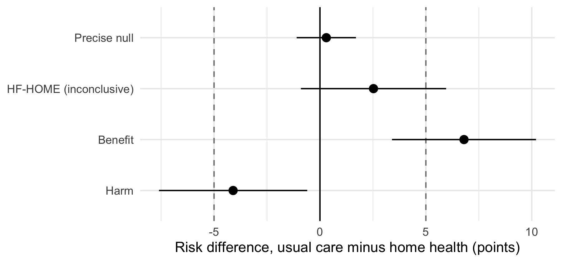
| Pattern | Where the interval sits | What you may claim |
|---|---|---|
| Precise null | Inside \((-\text{MCID}, \text{MCID})\), including zero | No effect of clinically meaningful size; a real, publishable finding |
| Inconclusive | Includes zero and reaches past an MCID line | No evidence of an effect, and no evidence of its absence; name what the interval rules out |
| Benefit | Wholly above zero | A reduction; whether it is clinically important depends on where the lower limit sits relative to the MCID |
| Harm | Wholly below zero | An increase in risk, stated as plainly as a benefit would be |
33.2.2 What HF-HOME’s interval rules out
An inconclusive result is not empty. The interval excludes some effects, and saying which ones makes the report informative. HF-HOME’s interval rules out a benefit larger than 6.0 points and a harm larger than 0.9 points. It cannot rule out no effect, and it cannot rule out the 5-point reduction the trial was designed to detect. The sentence to write is: ‘the trial was inconclusive; its interval is consistent with no effect and with a reduction of up to 6.0 points, and excludes harms larger than 0.9 points’.
Contrast that with ‘the difference was not statistically significant (p = 0.15)’. That sentence tells the reader nothing about whether the study was informative, and it would read the same for a precise null.
33.2.3 An inconclusive result is not a failed study
Consider a trial that enrolled half its target and produced an interval spanning every effect from large harm to implausibly large benefit. That trial has produced no result, and the honest report says so. HF-HOME is not that trial. Both arms reached the 1,094 evaluable patients the SAP required (1,133 and 1,136), and the interval is about as narrow as the design promised. The observed reduction is about half the planned one, and a trial with 80% power misses an effect of the planned size one time in five. Its result is a properly sized estimate that happens to straddle the line. It will be worth more in a future meta-analysis than in a ‘negative’ headline.
WarningPitfall
‘No significant difference’ becomes ‘no difference’ in the abstract. Each revision of a draft shortens the sentence, and the shortest version of an inconclusive result is a negative one. Presenting an underpowered or inconclusive null as evidence of no effect is how the literature acquires ‘negative’ trials that were merely imprecise. The statistician is usually the only person on the team in a position to stop it. Check the abstract’s verb against Table 33.2 at every revision, not only the first.
WarningEthics
Overclaiming runs in both directions. Turning an inconclusive interval into ‘no effect’, or an observational association into ‘reduces’, says more than the evidence supports. The reader acts on the verb rather than the interval. Section 32.4 treats the causal verb as an ethical matter, not a stylistic one (Chapter 32).
33.2.4 Exercises
- Classify each interval (risk difference in points, positive is benefit) against an MCID of 5, then against an MCID of 2:
- 1.2, from -0.8 to 3.2; (b) 4.0, from 0.5 to 7.5;
- -2.0, from -6.5 to 2.5; (d) 0.3, from -3.9 to 4.5. Which classifications depend on the MCID?
NoteSolution
ex <- tibble(
  interval = c("a", "b", "c", "d"),
  lower    = c(-0.8, 0.5, -6.5, -3.9),
  upper    = c(3.2, 7.5, 2.5, 4.5)
) |>
  mutate(mcid_5 = classify_interval(lower, upper, 5),
         mcid_2 = classify_interval(lower, upper, 2))
ex
#> # A tibble: 4 × 5
#>   interval lower upper mcid_5       mcid_2
#>   <chr>    <dbl> <dbl> <chr>        <chr>
#> 1 a         -0.8   3.2 Precise null Inconclusive
#> 2 b          0.5   7.5 Benefit      Benefit
#> 3 c         -6.5   2.5 Inconclusive Inconclusive
#> 4 d         -3.9   4.5 Precise null Inconclusive
Intervals (a) and (d) are precise nulls against an MCID of 5 and inconclusive against an MCID of 2: both include effects larger than 2 points. Interval (b) excludes zero whatever the MCID, and (c) reaches past -5, so it is inconclusive under either. The MCID is therefore part of the claim, which is why the SAP names it before the data arrive. Chosen afterward, it can be set to make any interval a precise null.
NoteCheck
Question. Your trial estimates a treatment effect of 0.3 points with a 95% interval from -3.9 to 4.5, and the MCID agreed at the outset was 2 points. The PI would like to write ‘the intervention was not effective’. What do you say?
Answer. That the sentence is not supported. The interval includes effects as large as 4.5 points, more than twice the MCID. The data are therefore consistent with a clinically important benefit, and with a clinically important harm. The correct report is that the study was uninformative in the range that matters: ‘we found no evidence of an effect, but the study cannot exclude a clinically important benefit or harm’. The PI’s sentence would be defensible only if the interval lay wholly inside \((-2, 2)\).
33.3 What would change the conclusion
6.7% of HF-HOME’s patients have no ascertainable outcome. The complete-case estimate is valid if loss to the state health-information exchange is unrelated to the outcome given arm. No data can confirm that. The SAP’s section 11 therefore pre-specifies a two-dimensional tipping-point analysis (Section 21.6). Unascertained patients in each arm are assigned \(\delta\) times the risk of their observed peers in that arm. The two values, \(\delta_U\) (usual care) and \(\delta_H\) (home health), are varied independently from 0.5 to 2. The cell with \(\delta_U = \delta_H = 1\) is missing at random (MAR). Every randomized patient stays in the denominator. The report names every combination that would change the conclusion, in either direction.
33.3.1 The grid on the running study
The code is the same as the worked example in Section 21.6, with the same seed, so the two chapters report the same grid.
set.seed(20260423)
arms <- rates |>
  transmute(arm, n, n_mis = n_miss, events, n_obs)

tip_cell <- function(delta_usual, delta_home, m = 50) {
  draws <- replicate(m, {
    p <- rbeta(2, arms$events + 1, arms$n_obs - arms$events + 1)
    p_mis <- pmin(1, p * c(delta_usual, delta_home))
    risk <- (arms$events + rbinom(2, arms$n_mis, p_mis)) / arms$n
    c(est = risk[1] - risk[2], var = sum(risk * (1 - risk) / arms$n))
  })
  q_bar <- mean(draws["est", ])
  b <- var(draws["est", ])
  t_var <- mean(draws["var", ]) + (1 + 1 / m) * b
  df <- (m - 1) * (1 + mean(draws["var", ]) / ((1 + 1 / m) * b))^2
  half <- qt(0.975, df) * sqrt(t_var)
  100 * c(estimate = q_bar, lower = q_bar - half, upper = q_bar + half)
}

grid <- expand.grid(delta_usual = seq(0.5, 2, by = 0.25),
                    delta_home  = seq(0.5, 2, by = 0.25))
grid <- cbind(grid, t(mapply(tip_cell, grid$delta_usual,
                             grid$delta_home)))
grid$conclusion <- with(grid, ifelse(lower > 0, "Benefit",
                                     ifelse(upper < 0, "Harm",
                                            "Inconclusive")))

mar      <- grid[grid$delta_usual == 1 & grid$delta_home == 1, ]
benefit  <- grid[grid$conclusion == "Benefit", ]
n_harm   <- sum(grid$conclusion == "Harm")
min_gap  <- min(benefit$delta_usual - benefit$delta_home)
tip_usual <- min(benefit$delta_usual[benefit$delta_home == 1])

table(grid$conclusion)
#>
#>      Benefit Inconclusive
#>           10           39
benefit |> arrange(delta_home, delta_usual) |> head(10)
#>    delta_usual delta_home estimate     lower    upper conclusion
#> 1         1.25       0.50 3.527961 0.1079844 6.947937    Benefit
#> 2         1.50       0.50 4.072368 0.6123056 7.532431    Benefit
#> 3         1.75       0.50 4.475329 1.0184967 7.932161    Benefit
#> 4         2.00       0.50 4.830592 1.3861441 8.275040    Benefit
#> 5         1.50       0.75 3.636513 0.2163363 7.056690    Benefit
#> 6         1.75       0.75 4.111842 0.6310922 7.592592    Benefit
#> 7         2.00       0.75 4.490132 1.0203598 7.959903    Benefit
#> 8         1.75       1.00 3.718750 0.2246554 7.212845    Benefit
#> 9         2.00       1.00 4.103618 0.6254839 7.581753    Benefit
#> 10 2.00 1.25 3.845395 0.3270403 7.363749 Benefitggplot(grid, aes(delta_usual, delta_home, fill = conclusion)) +
geom_tile(color = "white") +
geom_text(aes(label = sprintf("%.1f", estimate)), size = 3) +
scale_fill_manual(values = c(Benefit = "#92c5de",
Inconclusive = "grey90",
Harm = "#f4a582"),
name = "Conclusion") +
labs(x = expression(delta[U] ~ "(usual care)"),
y = expression(delta[H] ~ "(home health)")) +
coord_equal() +
theme_minimal()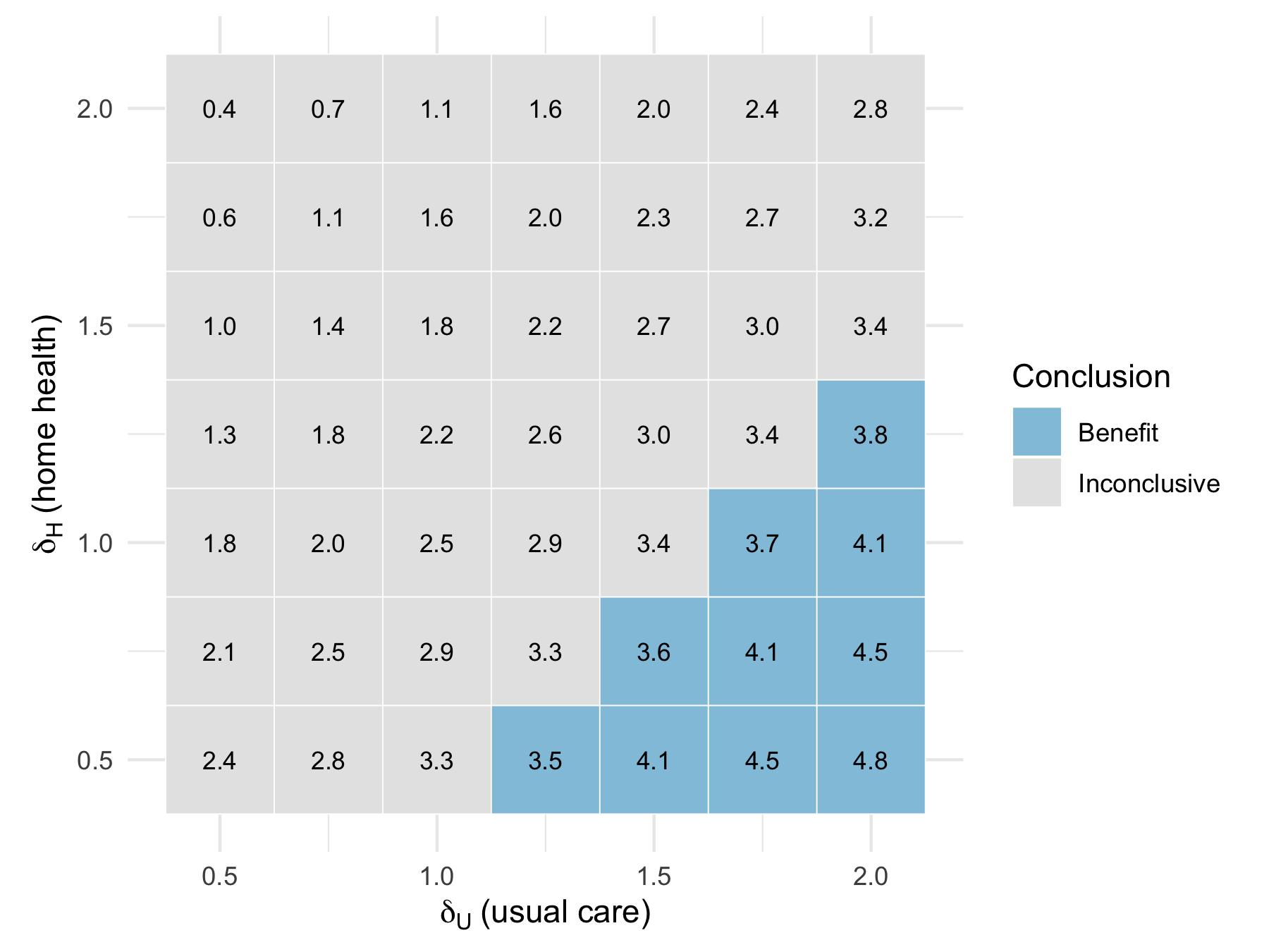
33.3.2 Reading the grid
Under MAR (the cell at 1, 1) the result is inconclusive, as the complete-case analysis is. Of the 49 combinations, 10 conclude benefit. In every one of them \(\delta_U\) exceeds \(\delta_H\) by at least 0.75. That is, unascertained usual-care patients would have to fare markedly worse than their observed peers, relative to unascertained home-health patients. Suppose home-health patients lost to the exchange fared like those retained (\(\delta_H = 1\)). Benefit then requires \(\delta_U \ge 1.75\), a 30-day risk of 41% among unascertained usual-care patients against 24% among those observed. The number of combinations that conclude harm is 0.
That is the paragraph the memo and the paper need. It is followed by one sentence of clinical judgment that no grid supplies. Loss to the exchange was driven by out-of-state addresses, and there is no known reason why patients who moved would fare worse on usual care than on home health. The analysis does not say which cell is true. A conclusion of ‘benefit’ in a corner of the grid is not a finding. It describes an assumption under which there would be one.
TipVerification
The MAR cell should reproduce the complete-case estimate, and every benefit cell should lie where \(\delta_U > \delta_H\), as the text claims:
WarningPitfall
A one-directional tipping-point rule reports ‘robust’ for a result with nothing to tip. An earlier version of the HF-HOME SAP raised \(\delta\) in the home-health arm ‘until the interval includes zero’. For an inconclusive result, the interval includes zero at the start. The rule stops at once, and a careless report calls the conclusion robust. A rule written on the assumption that the result will be positive is not pre-specified for the result you got. The two-dimensional grid answers the question for any result.
33.3.3 Beyond one grid: multiverse and specification-curve analysis
The tipping-point grid varies one assumption the SAP named in advance: the risk of unascertained patients relative to their observed peers. A related but distinct idea is to vary several analytic choices at once and report the distribution of results rather than a single preferred one. It is useful when each choice is individually defensible and none was pre-specified strongly enough to rule the others out. Specification curve analysis (Simonsohn et al., 2020) enumerates every combination of defensible choices (which covariates to adjust for, which exclusion criteria to apply, which link function to fit). It computes the estimate under each and plots the resulting curve of estimates, ordered from smallest to largest. It then tests jointly whether the pattern differs from what chance would produce. For HF-HOME, the primary estimator is pre-specified and the SAP already narrows the choice. The version of the idea that applies here is therefore narrower. We vary the covariate set used in the standardized estimator of the cumulative exercise, alongside the missingness assumption of the tipping-point grid. We then show whether the inconclusive conclusion survives every combination jointly, not just each dimension separately. A multiverse analysis is a transparency tool for choices that are genuinely contested. It does not substitute for pre-registering the one that matters most, and a trial with a tagged SAP has already made the harder commitment.
33.3.4 Exercises
- Using
gridandrates, find the combinations that conclude benefit when unascertained usual-care patients are assumed to fare exactly like their observed peers (\(\delta_U = 1\)). Then state, as a sentence for the memo, the smallest assumed risk among unascertained usual-care patients that produces benefit when \(\delta_H = 1\).
NoteSolution
No combination with \(\delta_U = 1\) concludes benefit. Lowering the assumed risk among unascertained home-health patients alone, even to half their peers’ risk, does not move the interval off zero. The sentence: ‘the result would become a benefit only if unascertained usual-care patients had a 30-day risk of 41% or more, against 24% among those we observed, while unascertained home-health patients fared like theirs’. Writing the risk, not \(\delta\), is what lets a clinician judge plausibility.
NoteCheck
Question. A collaborator reads Figure 33.3 and says ‘so under some assumptions it works’. What is wrong with the summary?
Answer. It reports a conditional as a finding. The grid shows which assumptions about unobserved patients would produce a benefit. Every such assumption requires usual-care patients lost to the exchange to fare much worse than home-health patients lost to it. There is no known mechanism for that. The accurate summary is that the inconclusive result does not hinge on the missing outcomes unless they are missing in a strongly arm-dependent way.
33.4 The memo
One page, to a principal investigator (PI), usually in answer to ‘what did you find?’ or ‘is this worth pursuing?’. The memo has a fixed shape. Its advantage is that the reader can stop at any point and still have something usable.
- The finding, in one sentence, with the number and its interval. No preamble.
- The request. What you want the reader to do: approve the manuscript, drop the arm, collect more data, stop.
- The three things they should know. The design in one line, the estimate in one line, the principal threat to it in one line.
- The caveats, ranked. The two or three that could actually change the conclusion, in descending order of how much.
- What you propose to do next, with a time cost.
Writing the memo is mostly a matter of cutting. Ask of each item ‘would the PI act differently if they knew this?’. Anything that fails the question comes out: most methods detail, the model specification, the diagnostics. They live in the compendium, and the memo says where. Every communication has an implicit request (fund this, publish this, stop this, collect more data, believe nothing yet). If you cannot state it, you are not ready to write. A PI will file and forget a memo that ends without one.
33.4.1 Before and after
The two versions below report the same analysis. The first follows the chronology; the second follows the five parts.
Before (chronological).
We received the final export on 2026-06-08. After cleaning, 2,269 of 2,432 patients had an ascertained outcome. Table 1 shows the arms were balanced. We fitted the pre-specified model and ran the sensitivity analyses. The 30-day risk was 23.7% with usual care and 21.1% with home health, a difference that was not statistically significant (p = 0.15). Next steps to be discussed.
After (answer first).
HF-HOME is inconclusive: home health lowered 30-day readmission or death by 2.5 points (95% CI -0.9 to 6.0), consistent with no effect and with the 5-point reduction we planned for. I recommend we publish it as inconclusive, not negative. The missing outcomes do not plausibly change this (see the tipping-point grid). I can draft methods and results in two weeks.
The first version is accurate, but it is of no use to a busy reader. The finding arrives in the sixth sentence, in the form a reader converts to ‘no effect’, and there is no request. The second gives the finding, its meaning, the recommendation, and the principal threat in four sentences.
33.4.2 Worked example: the HF-HOME memo
To: Dr. X, Cardiology From: A. Statistician Re: HF-HOME primary analysis, 2026-06-15
Finding. HF-HOME is inconclusive. Assignment to home-health visits within seven days of discharge lowered 30-day readmission or death by 2.5 percentage points (95% CI -0.9 to 6.0; from 23.7% to 21.1%). The interval includes both no effect and the 5-point reduction the trial was designed to detect.
Request. Approval to write the primary manuscript reporting the result as inconclusive, with the interval in the abstract, rather than as a negative or a positive trial; and to deposit the de-identified data (Chapter 34) so that the trial can enter future meta-analyses.
What you should know.
- Design: 2,432 patients, 1:1 randomized, stratified by site and ejection fraction, analyzed as pre-specified in SAP v1.0, tagged before unblinding. Both arms reached the 1,094 evaluable patients the plan required; this is not an underpowered trial.
- Estimate: the interval rules out a benefit larger than 6.0 points and a harm larger than 0.9 points. It cannot distinguish a 5-point benefit from none.
- Principal threat: 6.7% of patients had no outcome ascertainable from the state health-information exchange. In the pre-specified tipping-point analysis, 10 of 49 assumptions about those patients would produce a benefit, each requiring the usual-care patients lost to follow-up to fare much worse than the home-health ones; none produces harm.
Caveats, ranked.
- The missing outcomes above. I do not think an arm-dependent departure of that size is likely, because loss to the exchange is driven by out-of-state address rather than by illness, but it is the assumption the result rests on and the manuscript must say so.
- Open-label design. Readmission is close to a hard endpoint, but the decision to admit is a clinician’s judgment.
- Single health system. External validity is unaddressed.
Next. Draft methods and results in two weeks, with the interval plotted against zero and the 5-point MCID and the tipping-point grid as main-text figures (one day). I recommend no subgroup analyses beyond the pre-specified ejection-fraction strata.
Table 33.3 labels the five parts of the memo and the test each passes.
| Part | In this memo | The PI’s question it answers | Test |
|---|---|---|---|
| Finding | ‘Inconclusive’, the estimate, the interval, the MCID | What happened? | Readable alone, with the number and its meaning |
| Request | Publish as inconclusive; deposit the data | What do you want from me? | A decision the PI can make |
| What you should know | Design, what the interval rules out, the missing outcomes | Can I trust it? | Three lines, one threat |
| Caveats, ranked | Missing outcomes, open label, single system | What could change it? | Ordered by how much |
| Next | Draft in two weeks, two figures, no new subgroups | What happens now? | A time cost |
Notice what the memo leaves out: the model formula, the covariate list, the diagnostics, Table 1, the software versions. It points to the compendium, where all of that lives. It contains every fact on which the PI’s decision turns. It also says what the interval cannot rule out. A PI who learns that from a reviewer instead of from you will not trust the next memo.
ImportantLLM prompt
Context. I am writing a one-page memo to a clinical PI on a two-arm trial. Attached: the estimate and 95% interval for the risk difference, the MCID from the SAP, the share of missing outcomes, and the conclusion of each cell of a pre-specified tipping-point grid. The result is inconclusive.
Constraints. Use five parts in this order: finding, request, three things to know, ranked caveats, next steps with a time cost. Do not use ‘significant’, ‘trend’, ‘demonstrates’, ‘failed’, or ‘negative’. Do not introduce any number I did not supply.
Criteria. The first sentence states the estimate, the interval, and what the interval rules out. Each claim is licensed by the interval under Table 33.2. The memo fits on one page.
Failure mode. Calibration. The model reaches for ‘a trend toward benefit’ or ‘did not reduce’ where the evidence supports ‘consistent with no effect and with a benefit up to’. It also softens or drops the caveat that is least welcome. Check. For each sentence that makes a claim, find the row of Table 33.2 that licenses it. Then give the memo to a colleague and ask what you found and what you want. Send the summary numbers, never patient rows (Section 12.3). Before the draft leaves your hands, replace every number in it with the inline code that computes it.
33.4.3 Exercises
- Rewrite this paragraph answer-first, keeping every fact: ‘We obtained the registry extract in March and excluded 41 patients with missing discharge dates. A Cox model adjusted for age and sex was fitted. The hazard ratio for readmission with the new protocol was 0.82 (95% CI 0.70 to 0.96). We therefore recommend the protocol be continued while we examine the excluded patients.’
NoteSolution
‘Readmission was lower under the new protocol (hazard ratio 0.82, 95% CI 0.70 to 0.96), and I recommend continuing it. The estimate is adjusted for age and sex; 41 patients with missing discharge dates were excluded, and I am checking whether they differ before we report.’ The finding and the request now lead. The exclusion, which could change the conclusion, becomes the ranked caveat. The date of the extract and the model name move to the compendium. The verb stays ‘was lower’, not ‘reduced’, because a registry comparison does not license the causal verb (Chapter 32).
NoteCheck
Question. You sent a memo three weeks ago quoting a hazard ratio of 0.71. Rerunning after a data correction gives 0.78, which does not change the conclusion. Do you tell the PI, and what do you send?
Answer. Yes, promptly, even though the conclusion holds. The figure is already in circulation, in a slide deck or a draft, and every downstream use of 0.71 is now wrong. Someone else will find it. A discrepancy found by a reviewer costs far more than one you reported. Most important, you are establishing what your silence means. Suppose a collaborator learns that you report changes only when they alter conclusions. That collaborator must then verify everything, because your silence carries no information. Send the old number, the new number, what changed in the data, which commit produced each, and one sentence saying the conclusion is unaffected. Your value to a team is that your numbers can be relied on. That depends more on how you handle the ones that change than on the ones that do not.
33.5 The talk
Twenty minutes, a clinical audience, most of whom will not remember a number.
The first two minutes carry the talk. Deliver the and/but/therefore. If the audience leaves after two minutes they should have the finding. Everything after is for those who want to know whether to believe it.
One idea per slide, and the idea is the title. A slide titled ‘Results’ says nothing. A slide titled ‘Home health: between no effect and a 6-point reduction; the trial cannot tell which’ states the point. The figure beneath it is the evidence for the title. A listener who reads only the titles should get the argument.
Show the estimate with its uncertainty, once, and large. For HF-HOME that is the inconclusive row of Figure 33.2 on its own: the point and interval, a line at zero, and the MCID marked, drawn with geom_pointrange() as in Chapter 20. It is the single most important object in the talk. Do not bury it in a regression table, and do not show a regression table unless someone asks.
Anticipate the three questions. For almost any clinical analysis they are the same. How did you handle the patients who dropped out? Could this be confounding? Does it hold in the subgroup I care about? Have a backup slide for each. For HF-HOME the first is Figure 33.3. A question answered in ten seconds from a backup slide does more for your credibility than the prepared talk.
Do not show code. The compendium is where the code lives, and the audience is not there to audit it. One line at the end, naming the repository and its digital object identifier (DOI), is enough.
NoteCheck
Question. A colleague’s slide shows HF-HOME’s estimate as a bar from zero to 2.5 with no interval, titled ‘Home health reduced readmissions’. Name the two problems.
Answer. The title claims a reduction the interval does not establish, and the figure removes the interval that would have shown this. The bar also invites the reader to compare lengths, as if 2.5 points were the effect, when any value from -0.9 to 6.0 is consistent with the data. A point-and-interval plot against zero and the MCID fixes both.
33.5.1 A plain-language summary
Many journals, funders, and institutional review boards now ask for a one-page summary written for the trial’s participants and the general public. It is separate from the technical abstract. The problem is the same as for the talk, matching the writing to the audience, but for readers one step further from the work. The words this chapter has used to be precise (‘interval’, ‘MCID’, ‘inconclusive’) are words a lay reader skims past. The method is the same and/but/therefore skeleton, rewritten in plain words rather than compressed. State what the study looked at, what the patients and families already believed, what was found, and what it means for someone deciding about home-health visits today. For HF-HOME it reads as something like: ‘We studied whether a nurse visiting people at home shortly after a hospital stay for heart failure helps them avoid another hospital stay or death. We compared people who were randomly assigned to get these visits with people who got usual care. We did not find a clear difference between the two groups, but the study also could not rule out a real benefit, so more research is needed before we can say whether home visits help.’ No number appears unless it is unavoidable, and no technical term appears unexplained. A reader with no statistical training should recognize both the finding and its uncertainty. Writing this summary after the memo, not before, keeps it accurate. The memo already states what the interval licenses. The plain-language version translates that sentence rather than re-deriving it from the raw numbers.
33.6 Publication and submission tables
A reviewer who wants to know whether randomization worked reads a manuscript’s Table 1 before its abstract. A reader deciding whether the trial’s population resembles their own patients reads it instead of the abstract. It is also the table most often built by hand, column by column, from a spreadsheet pivot. That is slower than the alternative. It also introduces the one error a reviewer always catches: a count in the table that does not match the flow diagram’s denominator.
gtsummary (Sjoberg et al., 2021) builds this table from one call on a tidy data frame. It is the same package used for the case study’s Table 1 at Chapter 30, and the reasons to use it carry over from a report to a submission. The table is reproducible from the compendium, and its counts are the counts the analysis used. A data correction regenerates it rather than requiring someone to re-type cells.
33.6.1 Worked example: HF-HOME’s baseline table
A journal’s Table 1 for a two-arm trial gives the baseline characteristics, by arm, of the randomized population rather than the analytic one. Every randomized patient belongs in it, whether or not their outcome was later ascertained (CONSORT item 15, (Moher et al., 2025)). The table below joins the randomization data to the baseline covariates used in the SAP’s standardized estimator (the same files as the cumulative exercise in this chapter). It then stratifies by arm.
library(gtsummary)

table1_data <- trial |>
  left_join(read_hf("demographics.csv") |>
              select(patient_id, age, sex),
            by = "patient_id", relationship = "one-to-one",
            unmatched = "error") |>
  left_join(read_hf("baseline.csv") |>
              select(patient_id, ef_pct, discharge_med_count),
            by = "patient_id", relationship = "one-to-one",
            unmatched = "error")
stopifnot(nrow(table1_data) == nrow(trial),
          !anyNA(table1_data[c("age", "sex", "ef_pct")]))

table1_data |>
  select(arm, age, sex, ef_stratum, ef_pct, discharge_med_count) |>
  tbl_summary(
    by = arm,
    label = list(age ~ "Age (years)", sex ~ "Sex",
                 ef_stratum ~ "Ejection fraction stratum",
                 ef_pct ~ "Ejection fraction (%)",
                 discharge_med_count ~ "Discharge medications (n)"),
    statistic = list(all_continuous() ~ "{mean} ({sd})",
                      all_categorical() ~ "{n} ({p}%)"),
    missing_text = "Missing"
  ) |>
  add_overall() |>
as_kable()| Characteristic | Overall N = 2,432 | Usual care N = 1,216 | Home health N = 1,216 |
|---|---|---|---|
| Age (years) | 72 (11) | 72 (11) | 71 (11) |
| Sex | |||
| F | 1,066 (44%) | 553 (45%) | 513 (42%) |
| M | 1,366 (56%) | 663 (55%) | 703 (58%) |
| Ejection fraction stratum | |||
| Preserved EF | 1,215 (50%) | 608 (50%) | 607 (50%) |
| Reduced EF | 1,217 (50%) | 608 (50%) | 609 (50%) |
| Ejection fraction (%) | 42 (15) | 42 (15) | 41 (15) |
| Discharge medications (n) | 6.96 (2.66) | 6.92 (2.63) | 7.00 (2.68) |
Three choices in that call are the ones a reviewer checks. First, by = arm with no test added. A randomized trial’s baseline p-values test a hypothesis known to be true by design. The check callout later in this chapter (Table 33.7) treats including them as the defect. Second, missing_text = "Missing" keeps a visible row for any covariate with incomplete data, rather than silently shrinking the denominator. A Table 1 that drops missing rows without saying so understates the enrolled population. Third, the label argument renames variables once, centrally. The alternative is relabeling the printed table by hand after the fact, which is the step most likely to drift from the data when the model changes.
33.6.2 From draft table to submission format
as_kable() is the right call while drafting, because it renders identically in HTML and PDF output from the same .qmd source. At submission, most journals want either a Word table (as_flex_table() from the flextable extension) or the exact column order and footnote style their template specifies. Check the journal’s author guidelines for footnote conventions (abbreviations spelled out, units in the row label rather than a footnote) before the final render. Reformatting a gtsummary object is faster than rebuilding a hand-made one, but it is not free. Whichever output format you choose, the input data frame, the join, and the assertion above do not change. The table a reviewer receives is built from the same one validated in this chapter.
The in-house zztable1 package is not used in this book’s worked examples, for a specific and documented reason. As of this writing it leaves the missing-value row blank instead of reporting a count (Appendix C). That is the exact defect this section’s worked example avoids by using gtsummary. The statement concerns the current state of one package, not formula-interface tables in general. It should be re-checked before any submission that depends on it.
NoteCheck
Question. A collaborator asks why Table 1 reports age as mean (SD) rather than median (first quartile, third quartile), when Chapter 30 used the median for every continuous variable. What determines the choice, and where should it be made?
Answer. The shape of the variable in this sample, not a house style. A roughly symmetric variable like age is well summarized by the mean and SD. A skewed one, like the penguins’ body mass or a trial’s length of stay, is better summarized by the median and interquartile range, which a long tail does not distort. The choice belongs in the statistic argument. It is made once and explicitly, so that it is visible in the code rather than guessed from the printed numbers. The all_continuous() default in tbl_summary() is the median unless overridden, which is why the override above is explicit.
33.6.3 Exercises
- Extend
table1_datato includesite, and produce the table stratified by arm and faceted by site usingtbl_strata(). Which covariate’s balance would you report in the main text if a reviewer asked whether randomization was stratified correctly, and why?
NoteSolution
site_data <- table1_data |>
  left_join(read_hf("randomization.csv") |> select(patient_id, site),
            by = "patient_id", relationship = "one-to-one",
            unmatched = "error")

site_data |>
  select(site, arm, ef_stratum) |>
  tbl_strata(
    strata = site,
    .tbl_fun = ~ .x |> tbl_summary(by = arm, missing_text = "Missing")
)| Characteristic |
Site A
|
Site B
|
Site C
|
Site D
|
Site E
|
|||||
|---|---|---|---|---|---|---|---|---|---|---|
|
Usual care N = 3501 |
Home health N = 3501 |
Usual care N = 2851 |
Home health N = 2861 |
Usual care N = 2491 |
Home health N = 2491 |
Usual care N = 1871 |
Home health N = 1861 |
Usual care N = 1451 |
Home health N = 1451 |
|
| ef_stratum | ||||||||||
| Preserved EF | 175 (50%) | 175 (50%) | 147 (52%) | 148 (52%) | 127 (51%) | 126 (51%) | 90 (48%) | 90 (48%) | 69 (48%) | 68 (47%) |
| Reduced EF | 175 (50%) | 175 (50%) | 138 (48%) | 138 (48%) | 122 (49%) | 123 (49%) | 97 (52%) | 96 (52%) | 76 (52%) | 77 (53%) |
| 1 n (%) | ||||||||||
ef_stratum, because the SAP named site and ejection-fraction stratum as the randomization strata (Chapter 26). Reporting its balance by arm within site is the direct check that stratification worked. Age or sex balance is a secondary, reassuring fact rather than the one the design promised.
33.7 Choosing a reporting guideline
CONSORT governs this chapter’s examples because HF-HOME is a randomized trial. In general, however, a reporting guideline is chosen by study design, and a mismatch is apparent to any reviewer who checks. The EQUATOR Network maintains the current list. Table 33.5 gives the mapping a biostatistician needs most often. Each row was checked against its own statement or the EQUATOR Network’s listing.
equator-network.org) before a submission; guideline numbers and scopes have changed as often as every few years.
| Design | Guideline | What it governs | Citation |
|---|---|---|---|
| Randomized trial, results | CONSORT 2025 | Flow diagram, baseline table, primary and harm outcomes, deviations from the SAP | (Moher et al., 2025) |
| Randomized trial, protocol | SPIRIT 2025 | What a protocol must specify before enrollment; the companion to the SAP (Chapter 26) | (Chan et al., 2025) |
| Observational study | STROBE | Design, setting, participants, and the confounding structure of a non-randomized comparison | (Elm et al., 2007) |
| Prediction model, including one built with machine learning | TRIPOD+AI | Development and validation of a model that predicts an individual outcome; see the worked checklist at Section 31.7 | (Collins et al., 2024) |
| Study that develops, tunes, prompts, or evaluates a large language model (LLM) | TRIPOD-LLM | Task definition, prompting or fine-tuning method, human oversight, and task-specific performance, extending TRIPOD+AI for generative models | (Gallifant et al., 2025) |
TRIPOD-LLM is itself recent (January 2025) and modular. A core set of items applies to any study involving an LLM. Additional items depend on whether the model was fine-tuned, prompted without modification, or evaluated as a diagnostic tool. A related 2025 guideline, CHART (the Chatbot Assessment Reporting Tool, published in BMJ Medicine and listed by the EQUATOR Network), covers a narrower design: studies that evaluate the health advice a chatbot gives. Neither guideline is written for an LLM used in a specific analytical task inside a study, such as literature screening or chart abstraction. For that role, check the EQUATOR Network’s current listing before citing a guideline in a manuscript.
The current version of any of these can be found in one place. The EQUATOR Network’s library (equator-network.org/reporting-guidelines) lists the current guideline for a design and its extensions (an AI extension, a pragmatic-trial extension, an abstract-only extension, and so on). It also lists the journal checklists that implement it. A guideline’s number changes less often than its content. CONSORT has been revised twice since its 2001 version, in 2010 and 2025. Each revision added items (the 2025 checklist, for example, adds an open-science section covering registration and data sharing). A manuscript written against the older checklist omits them, and often no one notices until a reviewer checks the date. Table 34.1 applies a caution to federal policy dates (Chapter 34), and the same caution applies here. Cite the version you actually used, by year, and not the guideline’s name alone. ‘CONSORT’ without a year could mean any of three checklists published since 2001.
Whatever the current list, a design maps to exactly one primary guideline, chosen before data are seen. This is the same pre-specification discipline Chapter 26 applies to the statistical model. A study with both a prediction model and a trial-style comparison, for instance, may owe a reader both a TRIPOD+AI checklist for the model and a CONSORT flow diagram for the comparison. Naming both at the protocol stage means a reviewer does not have to ask which one governs.
WarningPitfall
A reporting guideline chosen at submission, rather than at protocol registration, invites a result-driven choice. STROBE has no requirement to report a primary endpoint’s p-value prominently; CONSORT does. A team whose primary analysis disappointed can be tempted to describe a randomized trial’s secondary, descriptive comparison using STROBE’s looser framing. The guideline follows the design, not the result, and the SAP or protocol should name it before unblinding.
33.7.1 Exercises
- A team runs a retrospective cohort study using electronic health record data to estimate the association between a medication and a safety outcome, then separately develops a machine-learning risk score from the same cohort to flag future risk. Name the guideline, or guidelines, the manuscript should follow, and justify each.
NoteSolution
Two, for two different claims in the same paper. The association estimate is an observational comparison, so it is reported against STROBE: design, setting, eligibility, and the confounders adjusted for. The risk score is a prediction model, so its development and validation are reported against TRIPOD+AI, including the calibration and discrimination items Section 31.7 works through in full. Neither guideline substitutes for the other; a paper that reports only STROBE items for the risk score would omit calibration entirely, which a STROBE checklist does not ask for.
33.8 The response to reviewers
The manuscript comes back with three reviewers and eleven comments, of which five are statistical and land on you. The response letter is its own genre with strict conventions.
Quote every comment, respond to every comment, in order. Number them, reproduce the reviewer’s text verbatim in a distinguishable typeface, and place your response beneath it. An editor must be able to verify, without cross-referencing, that nothing was ignored; silence on a comment reads as evasion even when it was an oversight.
Say what changed and where. ‘We have added the requested sensitivity analysis (Methods, p. 8; Supplementary Table S6; Figure 3 revised).’ A response that agrees but does not say where the manuscript now reflects it forces the editor to hunt.
Concede quickly what should be conceded. If the reviewer is right, say so in one sentence, make the change, and move on. Defensive paragraphs attached to a concession make it look grudging and invite scrutiny of the rest.
Disagree on technical grounds, once, and without heat. State the technical reason, offer the analysis that demonstrates it, and stop. Do not restate the point three ways or imply that the reviewer failed to read the paper, even when they plainly did not.
Do not let a request change the inferential status of an analysis. This is the statistical judgment at the center of the genre. A reviewer who asks for a subgroup analysis is asking for an analysis that was not pre-specified. Perform it, report it, and label it exploratory. The temptation, real because the reviewer holds the decision, is to fold it into the results as though it had been planned; the request does not launder the inference, and Chapter 26 exists to prevent exactly that. The same holds in the other direction: a reviewer who asks you to call an inconclusive trial negative is asking you to claim more than the interval licenses.
33.8.1 Worked example: four responses
Every number in the responses is computed. Those for Comment 1.3 come from the sensitivity chunk above. The subgroup figures for Comment 2.1 come from the chunk below, which splits the ascertained patients by the pre-specified ejection-fraction (EF) stratum.
by_stratum <- trial |>
  filter(ascertained) |>
  group_by(ef_stratum, arm) |>
  summarize(n_obs = n(), events = sum(event_30d), .groups = "drop") |>
  group_by(ef_stratum) |>
  summarize(
    rd = 100 * (events[1] / n_obs[1] - events[2] / n_obs[2]),
    se = 100 * sqrt(sum(events / n_obs * (1 - events / n_obs) /
                          n_obs)),
    .groups = "drop"
  )
stopifnot(identical(levels(trial$arm)[1], "Usual care"))

rd_reduced   <- by_stratum$rd[by_stratum$ef_stratum == "Reduced EF"]
rd_preserved <- by_stratum$rd[by_stratum$ef_stratum == "Preserved EF"]
z_int <- (rd_reduced - rd_preserved) / sqrt(sum(by_stratum$se^2))
p_int <- 2 * pnorm(-abs(z_int))

# The reviewer's premise, which the response below concedes
stopifnot(rd_reduced > rd_preserved)
by_stratum
#> # A tibble: 2 × 3
#>   ef_stratum      rd    se
#>   <chr>        <dbl> <dbl>
#> 1 Preserved EF  1.99  2.20
#> 2 Reduced EF    3.07  2.66
round(c(z = z_int, p = p_int), 2)
#>    z    p
#> 0.31 0.76
Comment 1.3. ‘The authors should report a sensitivity analysis to the missing outcome data, which at 6.7% is not negligible.’
We agree. The two-dimensional tipping-point analysis was pre-specified in SAP v1.0 (section 11) but reported only in the supplement; we have moved it to the main text (Results, p. 12; Figure 3). Unascertained patients remain in the denominator, and in each arm are assigned \(\delta\) times the risk of their observed peers, with the two \(\delta\)s varied independently from 0.5 to 2. Under missing at random the result is inconclusive, as in the primary analysis. 10 of the 49 combinations would conclude benefit, all with \(\delta\) for usual care exceeding that for home health by at least 0.75, and 0 would conclude harm. Since loss to follow-up was driven by out-of-state address rather than clinical status, we regard an arm-dependent departure of that size as unlikely, and the revised Discussion (p. 18) says so.
Comment 2.1. ‘The effect appears larger in patients with reduced ejection fraction. The authors should present this subgroup as a primary finding, as it is likely the mechanism.’
We have added the subgroup analysis (Supplementary Table S7). The point estimate is larger in the reduced-EF stratum (3.1 vs 2.0 points), and the test of interaction gives p = 0.76. We respectfully decline to present it as a primary finding. It was not pre-specified as one: the SAP, deposited before unblinding, names a single primary analysis in the full randomized population, and promoting a stratum chosen after seeing the data would make its error rate uninterpretable. The trial was also not powered for interaction, and a difference of this size between strata is well within what sampling variation produces under a common effect. We report it as exploratory (Results, p. 14).
Comment 2.4. ‘The primary analysis is not significant. The conclusion should state that home-health visits do not reduce readmission.’
We respectfully disagree, on the evidence. The 95% interval, -0.9 to 6.0 points, includes the 5-point reduction the trial was designed to detect, so the data do not exclude a clinically important benefit; ‘do not reduce’ would require an interval inside the range of clinical indifference. We have revised the Conclusion (p. 20) to state what the interval rules out (benefits larger than 6.0 points and harms larger than 0.9 points) and what it cannot.
Comment 3.2. ‘A logistic regression is inappropriate here; the authors should have used a Cox model.’
The outcome is binary readmission or death within a fixed 30-day window. Every patient linked to the state exchange is observed for the full window, and death is part of the outcome rather than a competing event. The 6.7% who could not be linked have a missing outcome, not a censored follow-up time, and are addressed in our response to Comment 1.3. There is no censoring to accommodate, and the estimand is a risk difference over a fixed horizon rather than a hazard ratio. We have added a sentence to the Methods (p. 7) making the estimand explicit.
Table 33.6 summarizes the four postures. None is defensive, and each tells the editor where to look.
| Comment | Posture | Response in one line | Change made |
|---|---|---|---|
| 1.3 Missing-data sensitivity | Concede | Pre-specified; now in the main text, with the cells that would tip | Results p. 12, Figure 3, Discussion p. 18 |
| 2.1 Promote the subgroup | Perform, decline to reframe | Reported as exploratory; not pre-specified, not powered | Table S7, Results p. 14 |
| 2.4 Call the trial negative | Defend | The interval includes the planned effect | Conclusion p. 20 states what is ruled out |
| 3.2 Use a Cox model | Defend | No censoring; the estimand is a fixed-horizon risk difference | Methods p. 7 |
The first response was cheap to write because of infrastructure built earlier. The sensitivity analysis existed because the SAP pre-specified it. Promoting its figure took a day because the compendium rebuilds with one command. The claim that the plan predates unblinding is verifiable because the SAP was tagged in Git (Chapter 26) and deposited at the registry. This is where the infrastructure chapters of this book repay the effort, six months after you last thought about the analysis.
ImportantLLM prompt
Context. Attached: one reviewer comment, verbatim; the relevant results with their intervals; the SAP section that pre-specifies (or does not pre-specify) the requested analysis; and my posture, which is one of concede, perform but decline to reframe, or defend.
Constraints. Write the response in under 150 words. Keep my posture; do not change it. Name the page, table, or figure that changed. No adjectives about the reviewer.
Criteria. Each technical claim cites the SAP section or the result that supports it. A concession is one sentence plus the change; a defense states the reason once.
Failure mode. The model tends to agree, and it concedes points it should defend. Typically it agrees to promote an exploratory subgroup, or to call an inconclusive trial negative, because the reviewer asked. Less often it writes a defensive paragraph where one sentence would do. Check. Compare each draft’s posture with the one you assigned in a table like Table 33.6. For each conceded point, ask whether you actually agree. For each defended point, ask whether the defense is technical rather than rhetorical.
33.8.2 Exercises
- Assign a posture (concede, perform but decline to reframe, or defend) to each comment, with one sentence of reason:
- ‘Please report the number of patients screened but not randomized.’ (b) ‘Please add a per-protocol analysis restricted to patients who received a visit, which better reflects the effect of the intervention.’ (c) ‘The tipping-point grid should extend to \(\delta = 3\).’
NoteSolution
- Concede: CONSORT requires the flow diagram to report it (Moher et al., 2025), and it costs a sentence. (b) Perform but decline to reframe: report it as a supplementary, exploratory analysis, and say why it cannot replace the primary. Patients who received the visit differ from those who did not, and patients with an event before the planned visit could not receive it, so the comparison breaks randomization (Section 26.2).
- Concede if cheap, with judgment stated. Extending the grid is one argument to
seq(). However, the response should say whether a tripled risk among patients lost to follow-up is clinically plausible. The grid’s range is a clinical claim, not a technical one.
NoteCheck
Question. In Comment 2.1 the response reports the interaction p-value. Why does it decline the reviewer’s request even if that p-value had been 0.03?
Answer. Because the objection is to the inferential status, not to the size of the p-value. A subgroup chosen after the data were seen, in a trial not powered for interaction, has an error rate no one can state. A small p-value from it is one draw from the garden of forking paths (Chapter 26). The response would report the p-value, label the analysis exploratory, and propose prospective testing.
33.9 Peer review as a practice
You learn the skills above by reviewing other people’s work more than by being reviewed. A reviewer who has had to explain why an analysis is unconvincing writes more convincing analyses. When reviewing a colleague’s analysis, ask the questions in Table 33.7, roughly in the order that catches the most.
| Question | Where to look | HF-HOME answer |
|---|---|---|
| What is the claim, in one sentence? | Abstract, first line of the memo | Inconclusive, with the interval |
| Is the interval interpreted, not merely printed? | Results, Conclusion | Yes: what it rules out is stated |
| Is the primary analysis the pre-specified one, verifiably? | The SAP tag and its date, not the prose | SAP v1.0 tag precedes unblinding |
| What is the denominator, and does it match the flow diagram? | Flow diagram, analysis code | All randomized in the sensitivity grid; ascertained in the complete case |
| Which assumption, if wrong, would most change the conclusion, and is it named? | Discussion, sensitivity analyses | Missing outcomes; the tipping-point grid |
| Could I re-run it? | The compendium, its lockfile, its build command | One command rebuilds every number |
For the statistical content specifically, the most compact published instrument is Harrell’s author checklist (Harrell, 2024). It enumerates errors a biomedical manuscript makes often enough to check mechanically: exact p-values rather than ‘NS’ or ‘p < 0.05’, intervals alongside tests, continuous variables not categorized, no stepwise selection, missingness documented rather than silently dropped, deviations from the analysis plan stated as deviations, and figures that show the data rather than a bar whose height is a mean. Run it against your own draft before you send it, which is cheaper than having a reviewer run it for you. Run it against a colleague’s draft when you review. Most of its items are failures of pre-specification that surface late enough to be expensive. A language model can provide a useful first pass. Ask it to review your results section as a hostile statistical reviewer and to list every claim the reported evidence does not support. It is better at finding overclaims in text than at avoiding them in its own. Treat each flag as a hypothesis to check against the analysis.
When receiving review, separate the comment from its tone. A reviewer who is rude and right has still given you a free defect report. The response letter is not the place to argue about the tone. The mildest version of a disagreement is almost always the most effective.
NoteCheck
Question. A draft you are reviewing reports ‘the groups were balanced at baseline (all p > 0.05)’ in Table 1 of a randomized trial. Which row of Table 33.7, or of Harrell’s checklist, does it touch, and what do you write?
Answer. It touches the interpretation of tests. In a randomized trial, baseline differences are chance by construction. P-values in Table 1 therefore test a hypothesis known to be true, and they say nothing about whether an imbalance matters. Write that the p-values should be removed. Any covariate whose imbalance could matter clinically is better handled by the pre-specified adjustment than by a test.
33.10 Rules of thumb
- Habit 11: lead with the answer, and match the verb to the design. An inconclusive answer goes first like any other, stated with what the interval rules out.
- Habit 10: every number in the prose is computed. The memo is where typed numbers survive longest; make its words as checkable as its numbers with an assertion on the pattern.
- Habit 5: pre-specify, then tag. A reviewer may ask for the subgroup, but cannot make it confirmatory; a sensitivity rule must be written to work whatever the result.
33.11 Cumulative practice
-
Cumulative (uses Chapter 26 and Chapter 18). The SAP’s primary estimator is not the complete-case difference above but a standardized one: a logistic regression of the outcome on arm, age, sex, ejection fraction, discharge medication count, and site, fitted to ascertained patients; predict every randomized patient’s risk under each arm, average, and take the difference, with a bootstrap percentile interval. Join the four files you need with declared relationships, compute the estimate, classify its interval with
classify_interval(), and say whether any sentence of the memo would change. - On your own work (no key). Take the last analysis you completed. Write its and/but/therefore in three sentences, then the five-part memo, and give it to a colleague who does not know the project. Ask them, without prompting, what you found and what you want them to do; revise until they can say both.
NoteSolution to exercise 7
covars <- read_hf("demographics.csv") |>
  select(patient_id, age, sex) |>
  left_join(read_hf("baseline.csv") |>
              select(patient_id, ef_pct, discharge_med_count),
            by = "patient_id", relationship = "one-to-one",
            unmatched = "error") |>
  left_join(read_hf("randomization.csv") |> select(patient_id, site),
            by = "patient_id", relationship = "one-to-one",
            unmatched = "error")

analytic <- trial |>
  left_join(covars, by = "patient_id", relationship = "one-to-one",
            unmatched = "error")
stopifnot(nrow(analytic) == nrow(trial),
          !anyNA(analytic[c("age", "sex", "ef_pct",
                            "discharge_med_count", "site")]))

standardized_rd <- function(d) {
  fit <- glm(event_30d ~ arm + age + sex + ef_pct +
               discharge_med_count + site,
             family = binomial, data = d[d$ascertained, ])
  risk <- vapply(levels(d$arm), \(a) {
    mean(predict(fit, newdata = mutate(d, arm = factor(
      a, levels = levels(d$arm))), type = "response"))
  }, numeric(1))
  100 * (risk[["Usual care"]] - risk[["Home health"]])
}

set.seed(20260423)
std_est  <- standardized_rd(analytic)
std_boot <- replicate(2000, standardized_rd(
  analytic[sample(nrow(analytic), replace = TRUE), ]))
std_ci <- quantile(std_boot, c(0.025, 0.975))

round(c(estimate = std_est, std_ci), 1)
#> estimate     2.5%    97.5%
#>      2.6     -0.8      6.1
classify_interval(std_ci[[1]], std_ci[[2]], mcid)
#> [1] "Inconclusive"
The standardized estimate is 2.6 points (95% bootstrap interval -0.8 to 6.1), close to the complete-case 2.5, as randomization implies. The covariate adjustment changes the precision a little and the conclusion not at all. The memo’s words therefore stand, and only its numbers would be replaced. We note that the bootstrap resamples all randomized patients and refits on the ascertained ones inside each resample. The averaging is therefore always over the full randomized population, as the SAP specifies. The relationship and unmatched arguments are what make the four-file join safe to trust without inspection.
33.12 Cheat sheet
| Task | Do | Guards against |
|---|---|---|
| Open any communication | The ‘therefore’ sentence: estimate, interval, meaning | A withheld conclusion |
| Report a null | Classify against zero and the MCID; say what is ruled out | ‘Not significant’ read as ‘no effect’ |
| Quote a number | Inline code, never typed | Stale numbers after a rerun |
| Guard the words |
stopifnot(pattern == "Inconclusive") before the memo |
Prose that outlives its result |
| Report missing-data sensitivity | Two-dimensional grid; name the cells that change the conclusion | A one-directional rule with nothing to tip |
| Write the memo | Finding, request, three facts, ranked caveats, next | A memo that is filed and forgotten |
| Show the estimate | Point and interval, zero and MCID marked | Bars and tables that hide uncertainty |
| Answer a reviewer | Quote, respond, say where it changed | An editor hunting for the change |
| Respond to a subgroup request | Perform, report, label exploratory | Laundering an exploratory result |
33.13 Further reading
- (Altman & Bland, 1995), the two-page paper this chapter’s null-results section restates at greater length.
- (Harrell, 2024), the author checklist used in the peer-review section.
- (Moher et al., 2025), the reporting standard that determines what a trial’s results section is obliged to state.
- (Gallifant et al., 2025), the current reporting guideline for studies that develop, prompt, or evaluate a large language model, used in Section 33.7.
33.14 Prerequisites answers
- Because the chronology withholds the conclusion until the end. It asks the audience to retain the preliminaries without yet knowing what they are for. An audience wants the claim first and the evidence second, so that they know what the evidence is evidence for. The chronology remains the right order for the methods section and for the compendium, where the reader’s purpose is verification rather than comprehension. For a talk or a memo, structure the material as an argument: the accepted state of the world, the disruption that motivated the work, the finding, the defense, and the conditions under which you would have concluded otherwise.
- ‘No evidence of an effect’ says that the study could not distinguish the effect from zero, a statement about the study’s resolution. ‘Evidence of no effect’ says that the effect is absent, or too small to matter, a statement about the world. You are entitled to the second only when the confidence interval excludes every effect you would have regarded as clinically meaningful. Such a precise null is a real and publishable finding. When the interval includes important effects, as HF-HOME’s does, the result is inconclusive, and the honest report names what the interval rules out and what it cannot.
- Three things, all argued for on other grounds. A pre-specified analysis plan tagged in Git before data lock (Chapter 26), so that you can show which analysis was primary and when it was fixed. A compendium that rebuilds with one command (Section 11.1, Chapter 11), so that changing the exclusion criterion is an edit and a re-render rather than a search through old files. And a pinned environment (Chapter 9, Chapter 10), so that the re-run six months later produces the published numbers rather than subtly different ones you then have to explain.