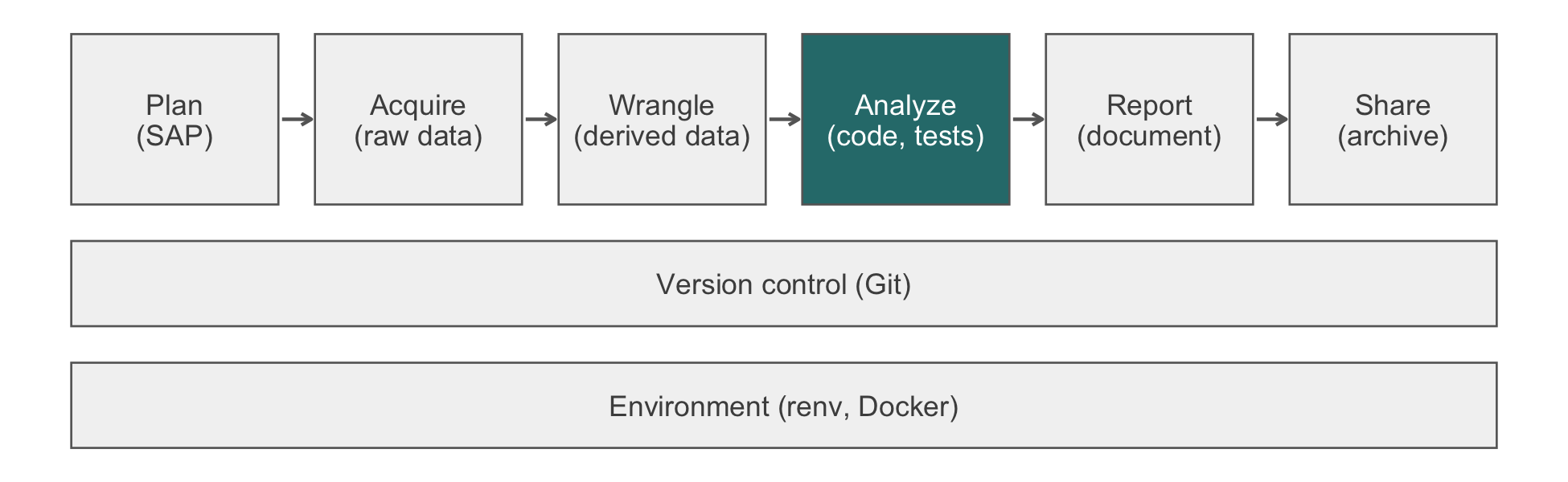
31 Case Study: ADNI MCI Prediction
A neurologist tells a 74-year-old woman and her daughter that the memory testing shows mild cognitive impairment (MCI). The daughter asks what every family asks: will it become Alzheimer’s disease, and how soon? An honest answer is a probability. The probability comes from a model fitted to a cohort like the Alzheimer’s Disease Neuroimaging Initiative (ADNI). Suppose that model counted the participants who left the study early as people who never progressed. Then the number the family hears is too low, and nothing in the code or its output says so. This chapter builds the compendium for such a model end to end. Each quiet decision is written down, pre-specified, and checkable by a reviewer who cannot see the data.
In God we trust; all others must bring data.
W. Edwards Deming, attributed; no source in his writings is known (in print by 1978)
NoteIn this chapter
Reading time. About 40 minutes.
You’ll need. Chapter 26 for the statistical analysis plan, Chapter 21 for complete-case reasoning, Chapter 4 for data-use agreements, Chapter 11 for the compendium, and Chapter 20 for trajectory plots. The code uses:
You’ll be able to.
- Derive an analytic cohort from longitudinal visits so that participants with an unobserved outcome are excluded or censored, never counted as non-converters, and report the count removed at each step.
- Pre-specify a prediction analysis (predictors, model, participant-level validation, discrimination, and calibration) and map it to the TRIPOD+AI reporting items.
- Run the whole pipeline against a synthetic stand-in, so that a reviewer without data access can verify the code.
- Structure a compendium whose code is public while its data stay under the data-use agreement.
Outline.
NoteSkip ahead?
If these answers come quickly, skip to the next chapter. The answers are in Section 31.12.
- What is the scientific question posed by the ADNI MCI prediction project, and why is it clinically meaningful?
- What features of the ADNI data make a reproducible compendium especially important relative to a typical pilot dataset?
- Why must ADNIMERGE data be preprocessed before modeling, and what preprocessing step is most commonly overlooked?
31.1 The question and the data
31.1.1 The research question
The case study predicts conversion from MCI to Alzheimer’s disease (AD) dementia within three years, from baseline sociodemographic, clinical, and neuropsychological measures. Solving the prediction problem would be a book-length exercise. The aim here is to demonstrate the workflow around it: scaffolding, planning, wrangling, describing, modeling, reporting, and depositing. The modeling itself is deliberately light. The companion book, Statistical Computing in the Age of AI, covers it.
From the statistical analysis plan (SAP), drafted with the template of Section 26.3:
Can baseline sociodemographic characteristics, clinical scales, and neuropsychological test scores predict conversion from MCI to AD dementia within 3 years?
Two secondary questions come from the same template. The first is which predictor categories (sociodemographic, clinical, neuropsychological) contribute most to prediction accuracy. The second is whether performance differs between early MCI (EMCI) and late MCI (LMCI).
MCI is a heterogeneous state. Some people progress to AD within months; others remain stable for years. Identifying those at highest risk enables targeted intervention trials, earlier counseling, and informed family planning. A model with modest discrimination is useful clinically. Here modest means an area under the receiver operating characteristic (ROC) curve, AUC, of 0.75 to 0.80. A model with an AUC of 0.95 has probably been trained or evaluated wrong. Prior work (Grassi et al., 2019) has established age, education, APOE4 status, and baseline ADAS13 as reliable predictors. The question is whether a multivariable model outperforms any one of them.
31.1.2 The ADNI dataset
ADNI is a longitudinal multicenter cohort study funded since 2004. Its data are obtained under a data-use agreement (DUA) at https://adni.loni.usc.edu/. The ADNIMERGE package is the community-standard R interface. It provides a single long-format table of roughly 15,000 visits on about 2,000 participants. Its more than a hundred variables span demographics, APOE genotype, clinical scales such as the Clinical Dementia Rating (CDR) and Functional Activities Questionnaire (FAQ), and neuropsychological tests.
| Variable | Description | Scale |
|---|---|---|
RID |
Participant ID | Integer |
VISCODE |
Visit code |
bl, m06, m12, … |
DX |
Diagnosis at the visit | CN (cognitively normal), MCI, Dementia |
DX_bl |
Baseline diagnosis | CN, SMC (subjective memory complaint), EMCI, LMCI, AD |
AGE, PTGENDER, PTEDUCAT
|
Age, sex, years of education | Demographics |
APOE4 |
Number of APOE $$4 alleles | 0, 1, 2 |
ADAS13 |
13-item Alzheimer’s Disease Assessment Scale, cognitive subscale: memory, language, praxis | 0 to 85, higher worse |
RAVLT.immediate |
Rey Auditory Verbal Learning Test, immediate recall: list learning | Higher better |
MMSE |
Mini-Mental State Examination: a cognitive screen | 0 to 30, higher better |
LDELTOTAL |
Logical Memory II delayed recall: story recall | Higher better |
APOE $$4 (apolipoprotein E, allele 4) is the most established genetic risk factor for late-onset AD. Relative to non-carriers, one copy raises risk roughly three-fold and two copies roughly eight- to twelve-fold in the large case-control meta-analyses, with estimates that vary by age, sex, and ancestry. The instruments are correlated but not redundant. Each captures a different aspect of cognition or risk. The predictive question is whether their combination outperforms any one alone.
NoteCheck
Question. A colleague reports a cross-validated AUC of 0.96 for three-year conversion from baseline measures alone. What is your first hypothesis?
Answer. That something leaks. The published range from baseline clinical and cognitive measures is far lower. MCI’s heterogeneity also limits how well any baseline profile can predict. Look first for an outcome-derived predictor (a variable measured after baseline). Then look for folds that split one participant’s visits across training and test.
31.2 Working under a data-use agreement
31.2.1 Why the compendium matters more here
ADNI analyses have three properties that make reproducibility both harder and more valuable. Each has an answer in the compendium.
| Property | Consequence | What the compendium does |
|---|---|---|
| Data-use agreement | The data cannot be shared | Public code, renv.lock, and a synthetic stand-in; collaborators obtain the data under their own DUA |
| Long time horizon | Reviewer requests and follow-up analyses arrive years later | A Docker-pinned environment reruns the original analysis on the same R and package versions |
Version churn in ADNIMERGE
|
New participants appear and variables are renamed between releases | The installed version recorded in renv.lock, the source tarball kept, and a frozen copy of the data file |
Data sharing is therefore asymmetric. The code can be public; the data cannot. The compendium ships in two parts. One is a public code-only deposit. The other is the documented route by which a collaborator obtains the data. The README states the distinction explicitly.
31.2.2 Scaffolding
Assemble the compendium by hand (Section 11.4) or with a framework. With the in-house zzcollab (Section 11.9), the session is (display-only):
mkdir adni-mci
cd adni-mci
zzc tidyverse            # scaffold the Five Pillars
make r                   # enter R inside the container
zzcollab has no modeling profile. Install the modeling packages inside the container: glmnet for penalized regression and survival for time-to-event handling of dropout. Record them with make snapshot, and rebuild the image with make docker-build.
ADNIMERGE is not on CRAN (the Comprehensive R Archive Network) or public GitHub. It is distributed as a source tarball through the LONI (Laboratory of Neuro Imaging) Image and Data Archive to investigators whose data-use application has been approved.1 Install the file you downloaded (display-only):
1 As of October 2026, ADNI also distributes a successor package, ADNIMERGE2; check which one your approval covers.
renv.lock now records the ADNIMERGE version, with a local rather than a repository source. renv::restore() cannot download it for a collaborator. Instead, each collaborator obtains the same tarball from LONI under their own DUA. They place it where renv looks for local sources (see ?renv::paths, RENV_PATHS_LOCAL). The restore then installs the same version.
Under analysis/, the compendium grows:
analysis/
├── data/
│   ├── raw/adnimerge_20260301.rds      # frozen copy, gitignored
│   └── derived/
│       ├── analytic_cohort.rds         # one row per RID
│       ├── adnimerge_clean.rds         # visits of the cohort
│       └── predictions.rds             # held-out predictions
├── paper/paper.qmd
└── scripts/
    ├── 00-simulate.R                   # the synthetic stand-in
    ├── 01-build-cohort.R
    ├── 02-table1.R
    ├── 03-trajectories.R
    └── 04-model.R
data/raw/adnimerge_20260301.rds is a frozen snapshot of the data on the date of analysis. The analysis therefore reruns against the same data even after ADNIMERGE updates. The file is gitignored. The README documents how a collaborator with DUA access recreates it.
WarningPitfall
Participant-level rows leave the enclave without an error. A head(adnimerge) pasted into a chat window, a CSV attached to an issue, or a data file committed and pushed to a public repository each discloses DUA-restricted data. Nothing in R, Git, or the chat interface stops it. The ADNI DUA limits the data to the uses in your approved application and forbids passing them on. A language-model service is a third party like any other. Send structure: column names, types, the schema of the synthetic stand-in, and aggregate summaries. Add the data directories to .gitignore before the first commit, not after the first push.
31.2.3 A synthetic stand-in
The real analysis cannot execute in this book, and a reviewer without a DUA cannot run it either. Both problems have the same answer. A generator produces data with the schema of ADNIMERGE, so that every script runs end to end without any ADNI file present. The generator below writes long-format visits for the five baseline diagnoses. Among the MCI participants, conversion to dementia depends on APOE4 dose, LMCI status, and baseline ADAS13. By default, dropout does not depend on anything. Only ADAS13 changes over time. The other measures are baseline values repeated, which is all the scripts need.
library(dplyr)

#' Simulate visit-level data with the ADNIMERGE schema
#'
#' @param n Number of participants.
#' @param seed Random seed.
#' @param dropout_rate Yearly dropout hazard; 0 means no dropout.
#' @param dropout_adas Log-hazard increase in dropout per ADAS13
#'   point above 15; 0 makes dropout uninformative.
#' @return A tibble with one row per visit.
simulate_adnimerge <- function(n = 1500, seed = 41, dropout_rate = 0.12,
                               dropout_adas = 0) {
  set.seed(seed)
  dx_bl <- sample(c('CN', 'SMC', 'EMCI', 'LMCI', 'AD'), n,
                  replace = TRUE, prob = c(0.25, 0.10, 0.25, 0.30, 0.10))
  apoe4 <- sample(0:2, n, replace = TRUE, prob = c(0.55, 0.36, 0.09))
  adas_bl <- pmax(0, round(rnorm(n, c(CN = 9, SMC = 9, EMCI = 12,
                                      LMCI = 18, AD = 30)[dx_bl], 5)))
  # conversion risk rises with APOE4 dose, LMCI, and ADAS13: the
  # associations the analysis is meant to find
  rate <- exp(-2.6 + 0.5 * apoe4 + 0.6 * (dx_bl == 'LMCI') +
                0.05 * (adas_bl - 15))
  t_convert <- ifelse(dx_bl %in% c('EMCI', 'LMCI'), rexp(n, rate), Inf)
  # scaling one draw keeps the same participants when the rate is 0
  t_drop <- rexp(n) / (dropout_rate * exp(dropout_adas * (adas_bl - 15)))

  tibble(
    RID = seq_len(n), DX_bl = dx_bl, APOE4 = apoe4,
    AGE = round(rnorm(n, 73, 7), 1),
    PTGENDER = sample(c('Male', 'Female'), n, replace = TRUE),
    PTEDUCAT = pmin(20L, pmax(6L, as.integer(round(rnorm(n, 16, 2.7))))),
    RAVLT.immediate = as.integer(pmax(0, round(rnorm(n, 45 - adas_bl, 8)))),
    MMSE = as.integer(pmin(30, pmax(18, round(30 - adas_bl / 6 +
                                               rnorm(n, 0, 1.5))))),
    LDELTOTAL = ifelse(runif(n) < 0.04, NA_integer_,
                       as.integer(pmax(0, round(rnorm(n, 14 - adas_bl / 2,
                                                      3))))),
    bl_date = as.Date('2010-01-01') + sample(0:2500, n, replace = TRUE),
    adas_bl = adas_bl, t_convert = t_convert, t_drop = t_drop
  ) |>
    tidyr::crossing(month = c(0, 6, 12, 24, 36, 48)) |>
    filter(month == 0 | month / 12 <= t_drop) |>
    mutate(
      years = month / 12,
      VISCODE = ifelse(month == 0, 'bl', sprintf('m%02d', month)),
      # ADNI visit windows: a scheduled visit can fall weeks early or late
      EXAMDATE = bl_date + round(month * 30.44) +
        ifelse(month == 0, 0, sample(-45:45, n(), replace = TRUE)),
      DX = case_when(
        DX_bl == 'AD' ~ 'Dementia',
        DX_bl %in% c('CN', 'SMC') ~ 'CN',
        years >= t_convert ~ 'Dementia',
        .default = 'MCI'
      ),
      DX = ifelse(month > 0 & runif(n()) < 0.05, NA, DX),
      ADAS13 = round(pmax(0, adas_bl + years * (1 + 0.8 * APOE4 +
                                                  3 * (years >= t_convert)) +
                            rnorm(n(), 0, 2.5)), 1)
    ) |>
    select(RID, VISCODE, EXAMDATE, DX_bl, DX, AGE, PTGENDER, PTEDUCAT,
           APOE4, ADAS13, RAVLT.immediate, MMSE, LDELTOTAL)
}

adnimerge <- simulate_adnimerge()
glimpse(adnimerge)
#> Rows: 7,297
#> Columns: 13
#> $ RID             <int> 1, 1, 1, 1, 2, 2, 2, 3, 3, 3, 3, 3, 4, 4, 4, 4, 4, 4, …
#> $ VISCODE         <chr> "bl", "m06", "m12", "m24", "bl", "m06", "m12", "bl", "…
#> $ EXAMDATE        <date> 2013-03-02, 2013-08-14, 2014-03-19, 2015-03-01, 2011-…
#> $ DX_bl           <chr> "LMCI", "LMCI", "LMCI", "LMCI", "SMC", "SMC", "SMC", "…
#> $ DX              <chr> "MCI", "MCI", "MCI", "MCI", "CN", "CN", "CN", "CN", "C…
#> $ AGE             <dbl> 83.2, 83.2, 83.2, 83.2, 77.0, 77.0, 77.0, 74.4, 74.4, …
#> $ PTGENDER        <chr> "Male", "Male", "Male", "Male", "Female", "Female", "F…
#> $ PTEDUCAT        <int> 18, 18, 18, 18, 15, 15, 15, 14, 14, 14, 14, 14, 17, 17…
#> $ APOE4           <int> 0, 0, 0, 0, 0, 0, 0, 1, 1, 1, 1, 1, 1, 1, 1, 1, 1, 1, …
#> $ ADAS13          <dbl> 14.4, 15.5, 20.0, 23.0, 4.0, 7.4, 0.3, 0.2, 0.2, 6.4, …
#> $ RAVLT.immediate <int> 48, 48, 48, 48, 36, 36, 36, 53, 53, 53, 53, 53, 34, 34…
#> $ MMSE            <int> 27, 27, 27, 27, 27, 27, 27, 30, 30, 30, 30, 30, 28, 28…
#> $ LDELTOTAL       <int> 7, 7, 7, 7, 8, 8, 8, 13, 13, 13, 13, 13, 11, 11, 11, 1…
TipVerification
The assertions, not the generator, are the deliverable. A reviewer needs to know the synthetic frame can stand in for the real one. That claim is made by checking it:
stopifnot(
  !anyDuplicated(adnimerge[c('RID', 'VISCODE')]),
  all(adnimerge$DX_bl %in% c('CN', 'SMC', 'EMCI', 'LMCI', 'AD')),
  all(adnimerge$DX %in% c('CN', 'MCI', 'Dementia', NA)),
  all(adnimerge$APOE4 %in% 0:2),
  all(adnimerge$MMSE >= 0 & adnimerge$MMSE <= 30),
  all(adnimerge$ADAS13 >= 0 & adnimerge$ADAS13 <= 85),
  inherits(adnimerge$EXAMDATE, 'Date'),
  all(table(adnimerge$RID[adnimerge$VISCODE == 'bl']) == 1)
)
Three rules apply to every generator of this kind. First, schema constraints (types, levels, ranges, one baseline per participant) matter more than distributions. Whether ADAS13 is realistic is irrelevant. Pretending otherwise invites the generator to be mistaken for a model of the disease. Second, build in the associations the analysis claims to find. A pure-noise generator runs the pipeline without exercising it. Third, never present synthetic output as a result. Every number computed from adnimerge in this chapter recovers parameters written into the generator. It checks the code and says nothing about Alzheimer’s disease.
NoteCheck
Question. A reviewer asks for ‘the data’ so that they can check your code. What can you send, and what can you not?
Answer. You can send the public compendium (code, renv.lock, Dockerfile, README) and the synthetic generator with its assertions. Together they let the reviewer run every script. You cannot send ADNI data, extracts, or derived participant-level files, however small, because the DUA does not permit it. A reviewer who needs the real data applies to ADNI and runs the same code.
31.3 Building the analytic cohort
31.3.1 From visits to one row per participant
In the real project, scripts/01-build-cohort.R begins (display-only):
Everything after that line runs unchanged against the synthetic adnimerge. The cohort logic is wrapped in a function so that it can be tested (exercise 5).
predictors <- c('AGE', 'PTGENDER', 'PTEDUCAT', 'APOE4', 'ADAS13',
                'RAVLT.immediate', 'MMSE', 'LDELTOTAL')

#' Derive the three-year conversion outcome for baseline MCI
#'
#' @param raw Visit-level data with the ADNIMERGE schema.
#' @param horizon_days Length of the outcome window.
#' @param tolerance_days How early a month-36 visit may fall and
#'   still close the window.
#' @return One row per baseline EMCI or LMCI participant, with
#'   `converted_by_3y`, `last_dx_days`, and `outcome_observed`.
build_cohort <- function(raw, horizon_days = 3 * 365.25,
                         tolerance_days = 90) {
  baseline <- raw |>
    filter(VISCODE == 'bl', DX_bl %in% c('EMCI', 'LMCI')) |>
    select(RID, all_of(predictors), DX_bl, EXAMDATE)

  visits <- raw |>
    filter(RID %in% baseline$RID) |>
    arrange(RID, EXAMDATE) |>
    group_by(RID) |>
    mutate(days_since_bl = as.numeric(EXAMDATE - first(EXAMDATE))) |>
    ungroup()

  followup <- visits |>
    group_by(RID) |>
    summarize(
      converted_by_3y = any(DX == 'Dementia' &
                              days_since_bl <= horizon_days,
                            na.rm = TRUE),
      last_dx_days    = max(days_since_bl[!is.na(DX)]),
      .groups = 'drop'
    )

  # outcome observed: converted within 3 years (whenever they left),
  # or followed through the 3-year visit without converting
  baseline |>
    left_join(followup, by = 'RID', relationship = 'one-to-one') |>
    mutate(outcome_observed = converted_by_3y |
             last_dx_days >= horizon_days - tolerance_days)
}

cohort <- build_cohort(adnimerge)

analytic_cohort <- cohort |>
  filter(outcome_observed) |>
  filter(if_all(all_of(predictors), \(x) !is.na(x))) |>
  mutate(converted_3y = converted_by_3y) |>
  select(RID, all_of(predictors), DX_bl, EXAMDATE, converted_3y)

stopifnot(!anyDuplicated(analytic_cohort$RID),
          !anyNA(analytic_cohort$converted_3y))

# long-format visits of the same participants, for trajectories
adnimerge_clean <- adnimerge |>
  filter(RID %in% analytic_cohort$RID) |>
  group_by(RID) |>
  mutate(
    years_since_baseline = as.numeric(EXAMDATE - min(EXAMDATE)) / 365.25,
    visit_month = as.integer(sub('^m', '', sub('^bl$', 'm0', VISCODE))),
    APOE4_any = factor(APOE4 > 0, levels = c(FALSE, TRUE),
                       labels = c('No APOE4 allele', 'Any APOE4 allele'))
  ) |>
  ungroup()

derived <- file.path(tempdir(), 'derived')
dir.create(derived, showWarnings = FALSE)
saveRDS(analytic_cohort, file.path(derived, 'analytic_cohort.rds'))
saveRDS(adnimerge_clean, file.path(derived, 'adnimerge_clean.rds'))
In the project, derived is analysis/data/derived. The non-obvious step is outcome_observed. A participant who converted within three years is a converter whether or not they stayed in the study afterward. A participant who has not converted counts as a non-converter only if followed through the three-year visit; one who left earlier without converting has an unobserved outcome.
The code excludes those participants. That is simple and common, and it removes the misclassification. However, it is not neutral. Converters who left early stay in, while non-converters who left early go. The excluded cohort therefore over-represents converters and overstates the three-year risk. It overstates it by less than counting dropouts as non-converters understates it (exercise 1 measures both). The alternative is a time-to-event analysis that censors early leavers at their last visit. That means a Kaplan-Meier estimate for the three-year risk, and a Cox or discrete-time model for prediction. Both are unbiased when dropout is unrelated to the risk of conversion. The SAP pre-specifies which approach is primary, and the other is a sensitivity analysis. The excluded count goes in the follow-up box of Figure 31.2.
WarningPitfall
Dropouts counted as non-converters lower the risk without an error. Skip the outcome_observed filter and every one of the 241 participants who left early without converting becomes a non-converter. On the synthetic data the three-year conversion proportion is then 25%, against 36% among participants whose outcome was observed. (Exercise 1 compares both with the truth.) Every model fitted to that outcome inherits the understatement. The code runs, the table looks plausible, and the family in the opening hears a number that is too low.
ImportantLLM prompt
Use a model to draft the inclusion and exclusion section of the SAP, and check it against the code.
Context. Below are the ‘Cohort definition’ template from my SAP and the variable table of the ADNIMERGE schema (names, types, levels; no data). The population is participants with baseline EMCI or LMCI; the outcome is a diagnosis of dementia at any visit within three years of baseline. Visits fall up to 90 days from schedule.
Constraints. Do not treat participants who leave before three years without converting as non-converters. Keep a participant who converted and then left as a converter.
Criteria. Write each criterion so that it maps to one filter in code. List, for each criterion, the count the manuscript must report. State the alternative to exclusion (censoring in a time-to-event analysis) and the question it answers instead.
Failure mode. Models often write ‘participants with at least three years of follow-up’, which wrongly excludes early converters who then left. Or they write ‘participants who did not convert were classified as stable’, which reintroduces the dropout bias. Check. Translate each drafted criterion into a filter, run it on the synthetic data, and compare its counts with Table 31.3. Then have a clinical collaborator read the draft. Send the template and the schema, never rows (Section 12.3).
31.3.2 The cohort flow
The analytic cohort is not the enrolled cohort. The gap between the two is itself a reportable result. Figure 31.2 traces the derivation in the manner of a CONSORT (Consolidated Standards of Reporting Trials) flow diagram. Table 31.3 gives the counts the code produced. Each exclusion is a number the manuscript must state, because a reader cannot judge selection bias without it.
flowchart TD
  A["ADNIMERGE roster<br/><i>all participants</i>"] --> B["Baseline EMCI or LMCI<br/><i>exclude CN, SMC, AD</i>"]
  B --> C["3-year follow-up or conversion<br/><i>exclude insufficient follow-up</i>"]
  C --> D["Key predictors observed<br/><i>exclude, or impute per SAP</i>"]
  D --> E["Analytic cohort"]
flow <- tibble(
  step = c('Roster', 'Baseline EMCI or LMCI',
           'Outcome observed within 3 years', 'Predictors complete'),
  n = c(n_distinct(adnimerge$RID), nrow(cohort),
        sum(cohort$outcome_observed), nrow(analytic_cohort))
) |>
  mutate(excluded = ifelse(is.na(lag(n)), '', format(lag(n) - n)))
knitr::kable(flow)| step | n | excluded |
|---|---|---|
| Roster | 1500 | |
| Baseline EMCI or LMCI | 803 | 697 |
| Outcome observed within 3 years | 562 | 241 |
| Predictors complete | 537 | 25 |
TipVerification
Confirm that every participant excluded for follow-up neither converted within the window nor reached the three-year visit, and that every participant kept satisfies one or the other.
NoteCheck
Question. A participant attends only the baseline and 12-month visits, then drops out, diagnosed MCI at both. How should they appear in the analysis of the three-year outcome?
Answer. They were observed event-free for one year, not three, so their three-year outcome is unknown. Treating them as a non-converter is wrong, and biases the risk downward. Two options remain. The first is to censor them at month 12 in a time-to-event analysis, which keeps the year they were observed. The Kaplan-Meier estimate at three years is then the three-year risk. The second is to exclude them, as the code does. The cohort then consists of participants who either converted within three years or were followed through the three-year visit. (A shorter threshold, such as 24 months, would readmit the problem.) The cost is the upward bias described above. The SAP names one option as primary and the other as a sensitivity analysis.
31.3.3 Exercises
- Compare four estimates of the three-year conversion risk on synthetic data where the truth is known: the proportion with no dropout at all (
dropout_rate = 0, the target); dropouts counted as non-converters; dropouts excluded; and the Kaplan-Meier estimate with dropouts censored. Average over 20 simulated cohorts so that the pattern is not one draw’s noise.
NoteSolution
km_risk <- function(raw, horizon_days = 3 * 365.25) {
  event_times <- raw |>
    filter(DX_bl %in% c('EMCI', 'LMCI')) |>
    arrange(RID, EXAMDATE) |>
    group_by(RID) |>
    mutate(days = as.numeric(EXAMDATE - first(EXAMDATE))) |>
    summarize(
      event = any(DX == 'Dementia', na.rm = TRUE),
      time = if (event) min(days[DX %in% 'Dementia'])
             else max(days[!is.na(DX)]),
      .groups = 'drop'
    )
  km <- survival::survfit(survival::Surv(time, event) ~ 1,
                          data = event_times)
  1 - summary(km, times = horizon_days)$surv
}

risk_estimates <- function(seed) {
  observed <- simulate_adnimerge(seed = seed)
  target <- build_cohort(simulate_adnimerge(seed = seed,
                                            dropout_rate = 0))
  sim_cohort <- build_cohort(observed)
  100 * c(
    target   = mean(target$converted_by_3y),
    naive    = mean(sim_cohort$converted_by_3y),
    excluded = mean(sim_cohort$converted_by_3y[
      sim_cohort$outcome_observed]),
    censored = km_risk(observed)
  )
}

risk <- rowMeans(sapply(1:20, risk_estimates))
round(risk, 1)
#>   target    naive excluded censored
#>     31.3     25.8     35.4     32.7
With no dropout every outcome is observed, so the first number is the target, 31.3%. Counting dropouts as non-converters gives 25.8%, far below it. Excluding them gives 35.4%, above it. Early converters who left are kept and early non-converters who left are not, so converters are over-represented. The Kaplan-Meier estimate, 32.7%, is closest. Censoring uses each participant’s observed time without guessing the outcome after it. Its remaining gap is small next to the other two errors. Censoring relies on dropout being unrelated to the risk of conversion, as it is in this generator. When that may not hold, rerun the comparison with dropout_adas = 0.08 and plan a sensitivity analysis accordingly.
31.4 Describing the cohort
31.4.1 Table 1
gtsummary (Sjoberg et al., 2021) builds the Table 1 from the analytic cohort. Two choices need stating. APOE4 is stored as 0, 1, 2. It is summarized as counts, not as a mean, so it is declared categorical. ADAS13 is right-skewed in MCI cohorts, so continuous variables are summarized as median and quartiles. That is gtsummary’s default.
library(gtsummary)

analytic_cohort |>
  mutate(converted_3y = factor(converted_3y, c(FALSE, TRUE),
                               c('Did not convert', 'Converted'))) |>
  tbl_summary(
    by = converted_3y,
    include = c(AGE, PTGENDER, PTEDUCAT, APOE4, ADAS13, MMSE, DX_bl),
    type = list(APOE4 ~ 'categorical')
  ) |>
  add_overall() |>
as_kable()| Characteristic | Overall N = 537 | Did not convert N = 342 | Converted N = 195 |
|---|---|---|---|
| AGE | 73 (69, 78) | 73 (69, 78) | 73 (69, 78) |
| PTGENDER | |||
| Female | 260 (48%) | 164 (48%) | 96 (49%) |
| Male | 277 (52%) | 178 (52%) | 99 (51%) |
| PTEDUCAT | 16 (14, 18) | 16 (14, 18) | 16 (14, 18) |
| APOE4 | |||
| 0 | 277 (52%) | 197 (58%) | 80 (41%) |
| 1 | 215 (40%) | 127 (37%) | 88 (45%) |
| 2 | 45 (8.4%) | 18 (5.3%) | 27 (14%) |
| ADAS13 | 15.6 (11.7, 19.5) | 14.4 (11.0, 18.6) | 17.4 (13.1, 21.5) |
| MMSE | |||
| 22 | 6 (1.1%) | 2 (0.6%) | 4 (2.1%) |
| 23 | 3 (0.6%) | 2 (0.6%) | 1 (0.5%) |
| 24 | 21 (3.9%) | 15 (4.4%) | 6 (3.1%) |
| 25 | 43 (8.0%) | 25 (7.3%) | 18 (9.2%) |
| 26 | 90 (17%) | 58 (17%) | 32 (16%) |
| 27 | 121 (23%) | 78 (23%) | 43 (22%) |
| 28 | 123 (23%) | 72 (21%) | 51 (26%) |
| 29 | 73 (14%) | 46 (13%) | 27 (14%) |
| 30 | 57 (11%) | 44 (13%) | 13 (6.7%) |
| DX_bl | |||
| EMCI | 221 (41%) | 171 (50%) | 50 (26%) |
| LMCI | 316 (59%) | 171 (50%) | 145 (74%) |
A descriptive Table 1 carries no row p-values. The in-house zztable1 package (Appendix C) offers a similar formula interface with journal styles (console, nejm, lancet, jama, bmj, simple). However, as of this writing it leaves the missing-value row blank instead of reporting the count where a variable like APOE4 has missing values. Use gtsummary until that is fixed. Whichever tool you use, match the target journal’s template.
31.4.2 Cognitive trajectories
The trajectory plot is a sanity check that the cohort behaves as the literature says it should. ggplot2 draws it from the visit-level data. The mean and a 95% confidence interval at each scheduled visit are computed first, so the plot shows exactly the numbers in the summary.
library(ggplot2)

trajectory <- adnimerge_clean |>
  group_by(APOE4_any, DX_bl, visit_month) |>
  summarize(mean = mean(ADAS13), se = sd(ADAS13) / sqrt(n()),
            n = n(), .groups = 'drop')

ggplot(trajectory, aes(visit_month, mean, color = DX_bl)) +
  geom_line() +
  geom_pointrange(aes(ymin = mean - 1.96 * se, ymax = mean + 1.96 * se),
                  size = 0.2) +
  facet_wrap(~ APOE4_any) +
  scale_color_brewer(palette = 'Dark2') +
  scale_x_continuous(breaks = c(0, 6, 12, 24, 36, 48)) +
  labs(x = 'Months since baseline', y = 'ADAS13 (higher is worse)',
       color = 'Baseline') +
  theme_minimal()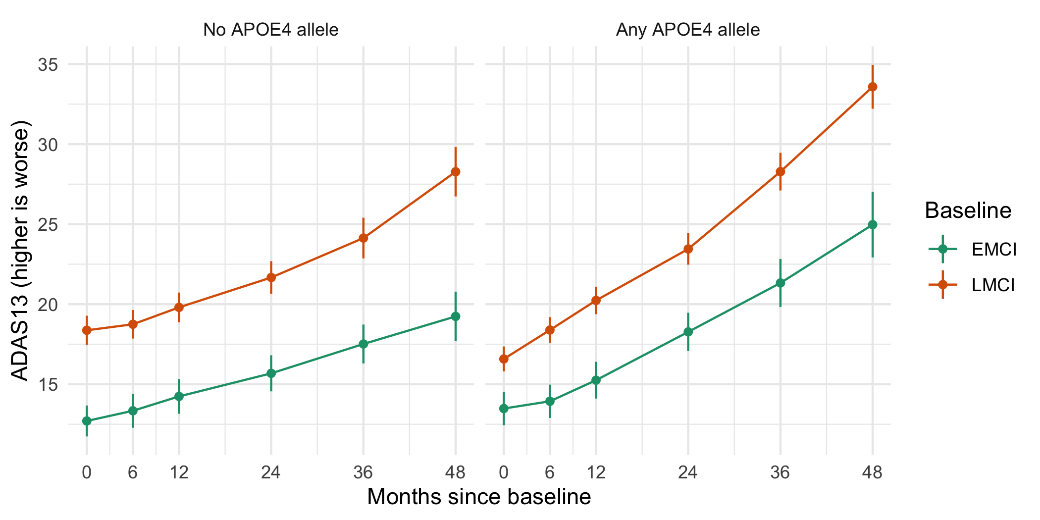
LMCI participants start worse than EMCI participants, and within each, APOE4 carriers worsen faster. Both observations are expected from the literature (and here, from the generator). If the real cohort did not show them, the cohort derivation would be the first suspect. The later visits average over fewer participants, the ones who stayed. That is the dropout problem again, in graphical form.
One way to automate a trial-style version of this figure is the in-house zzlongplot package (Appendix C). Its formula reads outcome by time, split by group after the bar. cluster_var names the column that identifies a participant (display-only):
zzlongplot::lplot(
  adnimerge_clean,
  form = ADAS13 ~ visit_month | DX_bl,
  facet_form = ~ APOE4_any,
  cluster_var = 'RID',
  summary_statistic = 'mean',
  confidence_interval = 0.95,
  clinical_mode = TRUE,
  theme = 'fda',
  xlab = 'Months since baseline',
  ylab = 'ADAS13'
)
theme selects a publication style (fda, nejm, lancet, jama, nature, science, jco).2
2 fda is the package’s label for a plain, high-contrast style intended for clinical study reports. The FDA (US Food and Drug Administration) publishes no figure style standard; its PDF specifications constrain page size, fonts, and resolution of submitted documents, not the look of a plot.
31.4.3 Exercises
- Add a second table to the compendium comparing baseline cognitive scores (
ADAS13,RAVLT.immediate,MMSE,LDELTOTAL) between EMCI and LMCI participants, with means and standard deviations, and produce it as both a Markdown and an HTML table.
NoteSolution
table_cog <- analytic_cohort |>
  tbl_summary(
    by = DX_bl,
    include = c(ADAS13, RAVLT.immediate, MMSE, LDELTOTAL),
    statistic = all_continuous() ~ '{mean} ({sd})'
  )
as_kable(table_cog)| Characteristic | EMCI N = 221 | LMCI N = 316 |
|---|---|---|
| ADAS13 | 13.1 (5.4) | 17.5 (5.5) |
| RAVLT.immediate | 32 (9) | 27 (9) |
| MMSE | ||
| 22 | 1 (0.5%) | 5 (1.6%) |
| 23 | 0 (0%) | 3 (0.9%) |
| 24 | 10 (4.5%) | 11 (3.5%) |
| 25 | 10 (4.5%) | 33 (10%) |
| 26 | 30 (14%) | 60 (19%) |
| 27 | 49 (22%) | 72 (23%) |
| 28 | 48 (22%) | 75 (24%) |
| 29 | 36 (16%) | 37 (12%) |
| 30 | 37 (17%) | 20 (6.3%) |
| LDELTOTAL | 8 (4) | 5 (3) |
html_file <- file.path(tempdir(), 'table-cognition.html')
gt::gtsave(as_gt(table_cog), html_file)
file.exists(html_file)
#> [1] TRUE
statistic overrides the default median and quartiles for every continuous variable at once. One tbl_summary() object renders to any format (as_kable(), as_gt(), as_flex_table() for Word), so the table is computed once and only its rendering differs. State in the caption which summary you used, because means and medians of a skewed score can differ by several points.
- Draw the ADAS13 trajectory stratified by three-year conversion rather than baseline diagnosis, and save it at 300 DPI (dots per inch) for journal submission.
NoteSolution
by_outcome <- adnimerge_clean |>
  left_join(select(analytic_cohort, RID, converted_3y), by = 'RID',
            relationship = 'many-to-one') |>
  group_by(converted_3y, visit_month) |>
  summarize(mean = mean(ADAS13), se = sd(ADAS13) / sqrt(n()),
            .groups = 'drop')

p <- ggplot(by_outcome, aes(visit_month, mean, color = converted_3y)) +
  geom_line() +
  geom_pointrange(aes(ymin = mean - 1.96 * se, ymax = mean + 1.96 * se)) +
  labs(x = 'Months since baseline', y = 'ADAS13',
       color = 'Converted by 3 years') +
  theme_minimal()

out <- file.path(tempdir(), 'adas13-by-outcome.png')
ggsave(out, p, width = 6, height = 4, dpi = 300)
dim(png::readPNG(out))
#> [1] 1200 1800    3
The saved file is 1,800 by 1,200 pixels, six by four inches at 300 DPI. Converters’ curves rise more steeply, as they must, because the outcome partly defines the trajectory. A plot stratified by an outcome measured later describes the outcome. It is not evidence that baseline measures predict it.
NoteCheck
Question. Why is APOE4 declared categorical in the Table 1 call, when it is a count?
Answer. A mean of 0.6 alleles describes no participant. It also hides the share of homozygotes, which is the clinically important group. As n (%) for 0, 1, and 2 alleles, the table shows the distribution a reader needs. gtsummary would treat a numeric column with three values as categorical anyway. Stating it makes the choice visible, and stable if a future extract has only two observed values.
31.5 The pre-specified analysis plan
ADNI is large and well studied, so an unprincipled analyst can find any signal they want in it. The SAP is written before the analytic cohort is opened (Chapter 26). It locks the predictor set, the model class, the validation strategy, and the metrics. Anything not pre-specified is exploratory. For ADNI, the SAP template of Section 26.3 has sections for background and rationale; research questions; cohort definition; exposure, outcome, and covariate definitions; the primary analysis; secondary analyses; missing-data handling; and sensitivity analyses. Table 31.5 separates what is locked from what is exploratory.
| Element | Pre-specified (locked before data access) | Exploratory (documented, not pre-specified) |
|---|---|---|
| Predictors | The eight baseline predictors in the cohort script, AGE through LDELTOTAL; no additions during model selection |
Variable-importance plot from the fitted model |
| Model | Penalized logistic regression with elastic net, tuning \(\alpha \in \{0, 0.5, 1\}\) and a grid of \(\lambda\) | Other model classes, reported as such |
| Validation | 10-fold cross-validation at the participant level; outer 80/20 holdout for final performance | Repeated or nested resampling |
| Metrics | AUC with bootstrap 95% confidence interval (CI; 1,000 resamples); calibration plot with calibration slope and intercept, as TRIPOD+AI expects | Decision-curve analysis |
| Threshold | Youden index on the training data, held fixed for evaluation; sensitivity, specificity, PPV, and NPV at that threshold | Alternative thresholds |
| Subgroups | None | Performance by EMCI and LMCI |
| Missing data | Complete case for predictors, with counts; dropout handled as in Section 31.3 | Multiple imputation as a sensitivity analysis |
The primary finding is valid because it was not selected after looking at the data. Tag the SAP commit before the cohort is built (Section 26.6), so that the order is provable.
ImportantLLM prompt
Draft the SAP’s missing-data section with a model, sending only an aggregate profile.
Context. Prediction model for three-year MCI-to-AD conversion; eight baseline predictors. Missingness profile (aggregate counts only):
LDELTOTALmissing in 4% of the cohort, other predictors complete; dropout before three years in about 30% of participants. No participant-level data are attached.Constraints. Do not recommend an approach by the fraction missing alone. Do not describe complete-case analysis as biased under MAR as a rule.
Criteria. For predictor missingness, state the condition under which complete case gives unbiased coefficients and what it costs in precision; specify multiple imputation with the outcome in the imputation model as the sensitivity analysis. Name at least one analysis of sensitivity to data missing not at random (MNAR). Handle dropout separately from predictor missingness.
Failure mode. Models recommend multiple imputation because ‘30% is a lot’. They call complete case biased whenever data are missing at random (MAR). Or they merge dropout (an outcome problem) with predictor missingness. Check. Compare the draft with Section 21.3. Complete case is unbiased for the coefficients when missingness does not depend on the outcome given the covariates, whatever the fraction. Check the DUA before sending anything, and send aggregates, never rows (Section 12.3).
NoteCheck
Question. After fitting the pre-specified model, you find that adding hippocampal volume raises the AUC by 0.04. Can it go in the primary analysis?
Answer. No. It was not in the locked predictor set. A predictor added after seeing performance turns the primary analysis into a selected one. Report it as exploratory, labeled as such, with the pre-specified model as the primary result. If it matters, it is the primary hypothesis of the next study’s SAP.
31.6 Modeling on the synthetic cohort
31.6.1 Participant-level validation
Cross-validation that splits at the observation level leaks information whenever a participant contributes several rows. The same person sits in training and test, and the AUC is optimistic in a way no held-out evaluation can match. The analytic cohort has exactly one row per RID, so ordinary fold assignment is already participant-level here. The rule matters as soon as a later visit enters the modeling frame. Then assign folds by RID, which in tidymodels is rsample::group_vfold_cv(group = RID). rsample::vfold_cv(strata = converted_3y) stratifies, preserving the class balance across folds, but it does not group.
The code below runs the pre-specified analysis with glmnet directly, assigning folds explicitly so that their level is visible. In the project it is scripts/04-model.R.
library(glmnet)

set.seed(2026)
test_rid <- analytic_cohort |>
  group_by(converted_3y) |>
  slice_sample(prop = 0.2) |>
  pull(RID)
train <- filter(analytic_cohort, !RID %in% test_rid)
test  <- filter(analytic_cohort, RID %in% test_rid)

design <- function(d) {
  model.matrix(reformulate(predictors), data = d)[, -1]
}
foldid <- sample(rep_len(1:10, nrow(train)))

fits <- lapply(c(0, 0.5, 1), \(a) {
  cv.glmnet(design(train), train$converted_3y, family = 'binomial',
            alpha = a, foldid = foldid)
})
best <- fits[[which.min(vapply(fits, \(f) min(f$cvm), numeric(1)))]]

p_train <- as.numeric(predict(best, design(train), s = 'lambda.min',
                              type = 'response'))
p_test  <- as.numeric(predict(best, design(test), s = 'lambda.min',
                              type = 'response'))

predictions <- tibble(RID = test$RID, observed = test$converted_3y,
                      predicted = p_test)
saveRDS(predictions, file.path(derived, 'predictions.rds'))
Storing the held-out predictions lets the figures and tables be regenerated without refitting, which matters when refitting is expensive.
31.6.2 Discrimination, calibration, and the threshold
auc <- function(y, p) {
  r <- rank(p)
  n1 <- sum(y)
  n0 <- sum(!y)
  (sum(r[y]) - n1 * (n1 + 1) / 2) / (n1 * n0)
}

auc_test <- auc(test$converted_3y, p_test)
auc_boot <- replicate(1000, {
  i <- sample(nrow(test), replace = TRUE)
  auc(test$converted_3y[i], p_test[i])
})

lp <- qlogis(p_test)
cal_slope <- coef(glm(test$converted_3y ~ lp, family = binomial))[['lp']]
cal_intercept <- coef(glm(test$converted_3y ~ offset(lp),
                          family = binomial))[[1]]

youden <- vapply(sort(unique(p_train)), \(t) {
  mean(p_train[train$converted_3y] >= t) +
    mean(p_train[!train$converted_3y] < t) - 1
}, numeric(1))
threshold <- sort(unique(p_train))[which.max(youden)]
flagged <- p_test >= threshold
y <- test$converted_3y

round(c(
  auc = auc_test, auc_lower = quantile(auc_boot, 0.025, names = FALSE),
  auc_upper = quantile(auc_boot, 0.975, names = FALSE),
  calibration_slope = cal_slope, calibration_intercept = cal_intercept,
  threshold = threshold,
  sensitivity = mean(flagged[y]), specificity = mean(!flagged[!y]),
  ppv = mean(y[flagged]), npv = mean(!y[!flagged])
), 2)
#>                   auc             auc_lower             auc_upper
#>                  0.70                  0.59                  0.80
#>     calibration_slope calibration_intercept             threshold
#>                  1.43                 -0.08                  0.40
#>           sensitivity           specificity                   ppv
#>                  0.59                  0.69                  0.52
#>                   npv
#>                  0.75
The AUC is computed in its rank-sum form. That is, it is the probability that a randomly chosen converter has a higher predicted risk than a randomly chosen non-converter. The calibration slope is the coefficient of the logit of the predicted risk in a logistic regression of the outcome on it. The calibration intercept is that regression’s intercept with the slope fixed at 1. A slope below 1 means the predictions are too extreme, and a slope above 1 means they are too cautious. Figure 31.4 shows calibration directly.
calibration <- predictions |>
  mutate(fifth = ntile(predicted, 5)) |>
  group_by(fifth) |>
  summarize(predicted = mean(predicted), observed = mean(observed),
            n = n(), .groups = 'drop') |>
  mutate(se = sqrt(observed * (1 - observed) / n))

ggplot(calibration, aes(predicted, observed)) +
  geom_abline(linetype = 'dashed', color = 'grey50') +
  geom_pointrange(aes(ymin = pmax(0, observed - 1.96 * se),
                      ymax = pmin(1, observed + 1.96 * se))) +
  coord_equal(xlim = c(0, 1), ylim = c(0, 1)) +
  labs(x = 'Mean predicted risk', y = 'Observed proportion converted') +
  theme_minimal()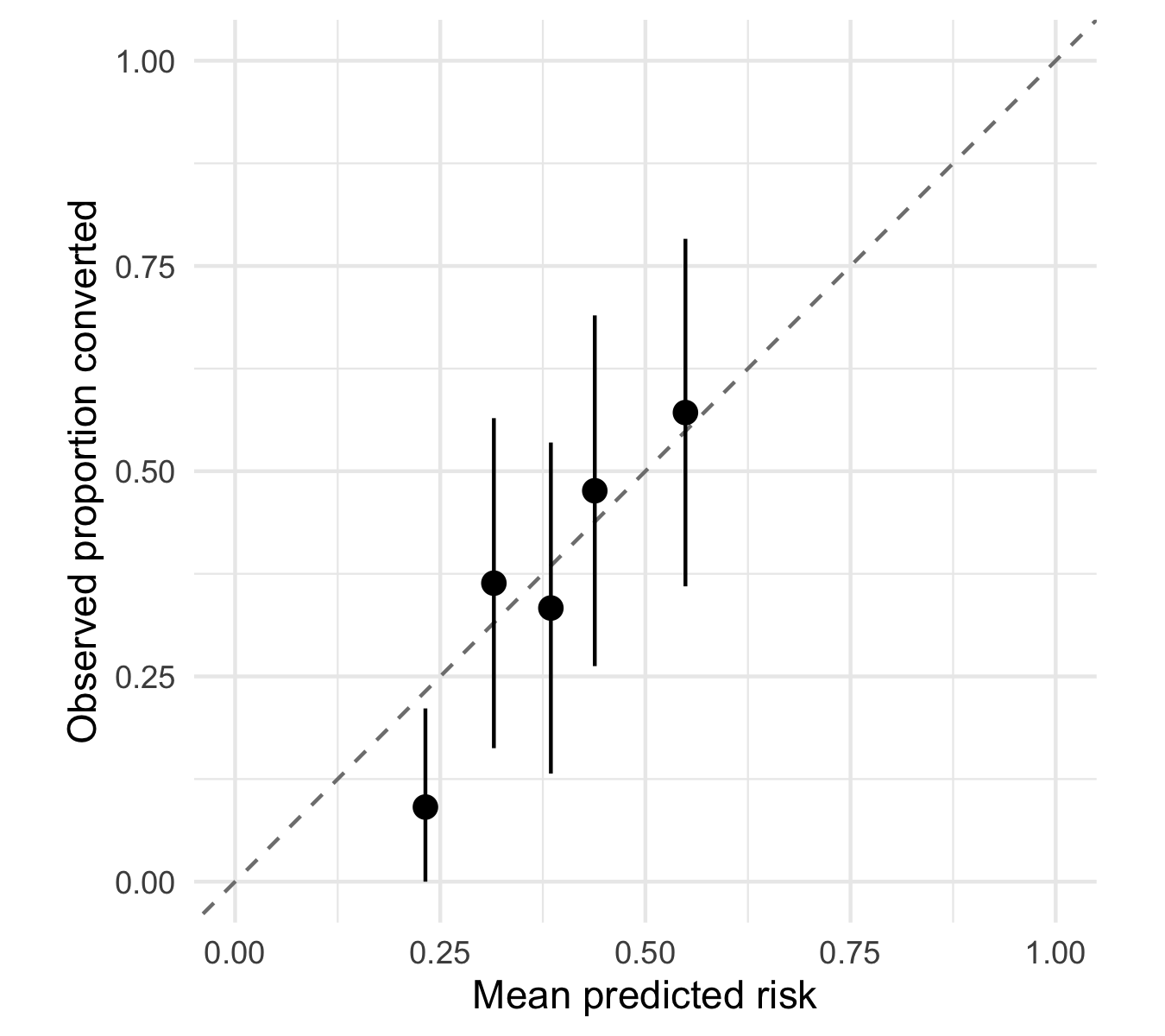
TipVerification
Confirm that no participant is in both the training and the test set, that the folds cover every training participant, and that the performance numbers come from the test set alone.
These numbers recover the generator’s parameters and are a check on the code. They are not evidence about Alzheimer’s disease, and must never be reported as such.
31.6.3 Exercises
- Suppose the modeling frame held every visit before month 12, several rows per participant. Assign ten folds at the participant level, and verify that no
RIDappears in more than one fold and that fold sizes are roughly equal.
NoteSolution
early_visits <- adnimerge_clean |>
  filter(visit_month < 12)

set.seed(7)
rid_fold <- tibble(RID = unique(early_visits$RID)) |>
  mutate(fold = sample(rep_len(1:10, n())))
early_visits <- left_join(early_visits, rid_fold, by = 'RID',
                          relationship = 'many-to-one')

folds_per_rid <- early_visits |>
  distinct(RID, fold) |>
  count(RID)
stopifnot(all(folds_per_rid$n == 1))
table(early_visits$fold)
#>
#>   1   2   3   4   5   6   7   8   9  10
#> 108 108 108 108 108 108 108 106 106 106
Folds are assigned to participants, then joined to visits, so a participant’s rows stay together. Fold sizes in rows vary a little, because participants contribute different numbers of visits. In participants they differ by at most one. Suppose you assigned sample(rep_len(1:10, nrow(early_visits))) to rows instead. Most participants’ two visits would then fall in different folds, and the stopifnot() would fail.
NoteCheck
Question. Observation-level folds on a frame with two visits per participant give an AUC of 0.88; participant-level folds give 0.74. Which do you report, and why is the first one higher?
Answer. Report 0.74. With observation-level folds, a participant’s second visit sits in the test fold while the first trained the model. The two visits are nearly identical, so the model is partly recognizing people it has seen. A new patient is never someone the model has seen. Only participant-level validation therefore estimates the performance the family in the opening would get.
31.7 Reporting and deposit
31.7.1 Reporting against TRIPOD+AI
The manuscript lives at analysis/paper/paper.qmd. Its frontmatter uses a journal format from a Quarto journal extension, installed with quarto use template or quarto add. (rticles provides the equivalent templates for R Markdown, not Quarto.) It takes the bibliography from references.bib. A prediction model is reported against TRIPOD+AI (Transparent Reporting of a multivariable prediction model for Individual Prognosis Or Diagnosis, updated for artificial intelligence). Its 27-item checklist supersedes TRIPOD 2015 for regression and machine learning models alike (Collins et al., 2024). Table 31.6 maps selected items, grouped by domain, to the place in the compendium that supplies them. The statement itself is the checklist to submit.
| Domain | What to report | Where the compendium supplies it |
|---|---|---|
| Title and abstract | Development of a prediction model with internal validation; population, predictors, outcome | paper.qmd |
| Data and participants | Source (ADNI phases, dates), eligibility, the flow with counts |
01-build-cohort.R; Table 31.3
|
| Outcome | Conversion within three years: definition, ascertainment, handling of incomplete follow-up | SAP; build_cohort()
|
| Predictors | The eight baseline predictors, defined and measured at baseline | SAP; Table 31.1 |
| Sample size | Participants and events in training and test |
Table 31.3; 04-model.R
|
| Missing data | Method and numbers excluded | SAP; Table 31.3 |
| Analysis | Model class, tuning, participant-level resampling, holdout | 04-model.R |
| Performance | Discrimination with CI; calibration plot, slope, intercept |
predictions.rds; Figure 31.4
|
| Fairness | Performance in relevant subgroups, such as sex | Exploratory analyses, labeled |
| Model specification | The fitted model in full, so that others can apply it | Coefficients at lambda.min
|
| Open science | Protocol or SAP, code availability, data access route | Zenodo deposit; README; the DUA route |
31.7.2 What gets deposited
| Deposit | Contents | Access |
|---|---|---|
| Zenodo (public) | Code, scripts, paper, README, Dockerfile, renv.lock, the synthetic generator with its assertions |
Open; this DOI is what the paper cites |
| Container registry | The built Docker image | Open; docker pull from the registry |
| ADNI | The data | Under the DUA only |
Collaborators with DUA access run the full analysis. Reviewers without it run every script against the synthetic generator. Make that the default. scripts/01-build-cohort.R should read the frozen ADNI file when it exists and call the generator in scripts/00-simulate.R when it does not. It should say which it used.
31.7.3 Verifying reproducibility
Before submitting, in a zzcollab project (display-only; the tool-neutral equivalents are in Section 11.7):
make check-renv-no-fix      # code, DESCRIPTION, and renv.lock agree
make docker-rebuild         # the image builds without the cache
make docker-render REPORT=analysis/paper/paper.qmd
Then, on a colleague’s machine: git clone, make docker-build, and the same render. Expect bit-identical output for the deterministic parts and rounding-level differences only where floating-point order matters.
NoteCheck
Question. A reviewer without ADNI access reruns your compendium and gets an AUC of 0.7, different from the paper’s. Is the compendium broken?
Answer. Not necessarily. They ran the synthetic generator, whose AUC reflects its own parameters. The check they can make is that every script runs and every assertion passes. The README should say this explicitly. The paper should never report a synthetic number, so that no reader can mistake one for the other.
31.8 Rules of thumb
- Habit 5: pre-specify, then tag. Lock predictors, model, validation, and metrics in the SAP, and tag it before the cohort is built.
-
Habit 8: a plausible number is the expensive bug. Dropouts counted as non-converters give a lower risk that looks entirely reasonable; the
outcome_observedfilter and its assertion make the choice loud. - Habit 12: send structure, not data. Under a DUA, the schema, the synthetic generator, and aggregates are all a model or a reviewer ever needs to see.
31.9 Cumulative practice
-
Cumulative (uses Chapter 27). Write a
tinytestfile forbuild_cohort()with a fixture of four synthetic participants: one who converted at month 24 and then left, one followed through month 36 without converting, one who left after month 12 without converting, and one who converted at month 48. Assertoutcome_observedandconverted_by_3yfor each.
NoteSolution
fixture_visits <- function(rid, months, dx) {
  tibble(
    RID = rid, VISCODE = ifelse(months == 0, 'bl',
                                sprintf('m%02d', months)),
    EXAMDATE = as.Date('2012-01-01') + round(months * 30.44),
    DX_bl = 'LMCI', DX = dx, AGE = 70, PTGENDER = 'Female',
    PTEDUCAT = 16L, APOE4 = 1L, ADAS13 = 18, RAVLT.immediate = 30L,
    MMSE = 27L, LDELTOTAL = 6L
  )
}
fixture <- bind_rows(
  fixture_visits(1, c(0, 12, 24), c('MCI', 'MCI', 'Dementia')),
  fixture_visits(2, c(0, 12, 24, 36), rep('MCI', 4)),
  fixture_visits(3, c(0, 6, 12), rep('MCI', 3)),
  fixture_visits(4, c(0, 12, 24, 36, 48),
                 c('MCI', 'MCI', 'MCI', 'MCI', 'Dementia'))
)
out <- arrange(build_cohort(fixture), RID)

library(tinytest)
expect_equal(out$converted_by_3y, c(TRUE, FALSE, FALSE, FALSE),
             info = 'only participant 1 converted within the window')
#> ----- PASSED      : <-->
#>  call| expect_equal(out$converted_by_3y, c(TRUE, FALSE, FALSE, FALSE),
#>  call| info = "only participant 1 converted within the window")
#>  info| only participant 1 converted within the window
expect_equal(out$outcome_observed, c(TRUE, TRUE, FALSE, TRUE),
             info = 'the early leaver without conversion is unobserved')
#> ----- PASSED      : <-->
#>  call| expect_equal(out$outcome_observed, c(TRUE, TRUE, FALSE, TRUE),
#>  call| info = "the early leaver without conversion is unobserved")
#>  info| the early leaver without conversion is unobserved
Participant 1 shows that an early converter who left stays in as a converter. Participant 3 shows that an early leaver without conversion is excluded. Participant 4 shows that a conversion after the window is a non-conversion within it, because the participant was followed through month 36. Each fixture row is a decision from the SAP, so the test file also serves as its executable specification.
-
On your own work (requires ADNI access, no key). With an approved DUA, run the compendium against
ADNIMERGEfor a different outcome (for example, progression from CN to MCI), adapting the SAP, the cohort function, and its tests, and deposit the code-only compendium with its synthetic generator.
31.10 Cheat sheet
| Task | Code | Guards against |
|---|---|---|
| Synthetic stand-in |
simulate_adnimerge() plus schema assertions |
Code no reviewer can run |
| Outcome observed | converted_by_3y \| last_dx_days >= horizon - tolerance |
Dropouts counted as non-converters |
| Cohort flow | Count after every filter()
|
Unreported selection |
| Table 1 | tbl_summary(by = ..., type = list(APOE4 ~ 'categorical')) |
Means of counts; row p-values |
| Participant-level folds | Assign folds to RID, then join; group_vfold_cv(group = RID)
|
Leakage across folds |
| Penalized model | cv.glmnet(x, y, family = 'binomial', foldid = foldid) |
Tuning on the test set |
| Discrimination | Rank-sum AUC with bootstrap CI | A point estimate without uncertainty |
| Calibration |
glm(y ~ qlogis(p), family = binomial); binned plot |
Discrimination reported alone |
| DUA | Schema and aggregates only, .gitignore the data |
Disclosure of participant rows |
31.11 Further reading
- (Collins et al., 2024), the TRIPOD+AI statement and checklist.
- (Weiner et al., 2017), an orientation to ADNI and its publication history.
- (Grassi et al., 2019), one example of the cohort-prediction approach this chapter sketches.
31.12 Prerequisites answers
- The question is: can baseline sociodemographic, clinical, and neuropsychological measures predict conversion from MCI to AD within three years? It is clinically meaningful because MCI is a heterogeneous state. Only some people progress to AD on a meaningful timescale. Identifying those at highest risk enables targeted intervention trials and earlier counseling.
- ADNI analyses carry three distinguishing features. The first is a data-use agreement that prevents data sharing, so the public compendium is code-only, with a synthetic stand-in. The second is a long time horizon: years pass between analysis and reviewer response, and the R ecosystem drifts meanwhile. The third is a dataset that updates periodically with renamed variables. All three increase the value of Docker-pinned environments and
renv-pinned package versions. - ADNIMERGE is long-format (one row per participant per visit), with mixed diagnostic labels and inconsistent visit codes across ADNI 1, GO, 2, and 3. Analytic cohorts require baseline-anchored follow-up windows, careful handling of participants who leave before the outcome window closes, and consistent visit alignment. The step most commonly overlooked is handling dropouts correctly. A participant who leaves after year 2 without converting has not been observed for the three-year outcome. Censor them in a time-to-event analysis, or exclude them and state that exclusion overstates the risk. Never treat them as non-converters.