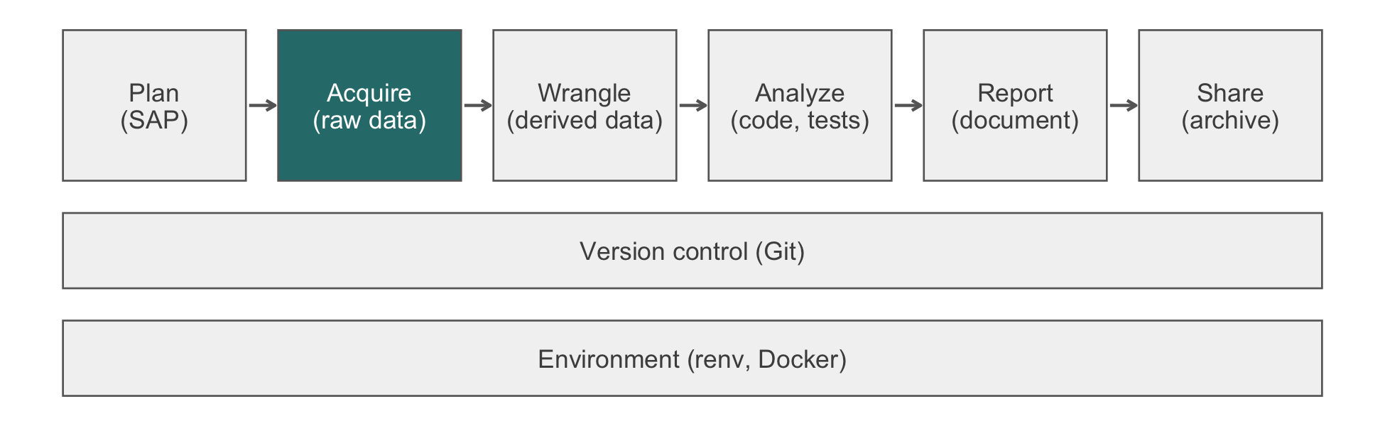
18  De-identification in Practice

Of the 2,432 patients in the HF-HOME demographics file, 2,422 are the only person in the file with their combination of five-digit ZIP code, date of birth, and sex, the three fields that singled out the Weld records (Chapter 4). The file is synthetic, but its fields behave as a real trial’s do, and the arithmetic is the same. Removing the names, record numbers, and telephone numbers changes none of those combinations. This chapter builds two releases of the file, one under Safe Harbor and one that needs an Expert Determination, writes the assertions each must pass, and then measures what both leave behind. The concepts are in Chapter 4; here they meet the wrangling and joins of the preceding chapters, and each claim about a release becomes a line of code that fails when the claim is false.

Data can be either useful or perfectly anonymous but never both.

Paul Ohm, Broken Promises of Privacy, UCLA Law Review (2010)

Figure 18.1: Where this chapter sits: a de-identified release is built at the Acquire stage, from the untouched raw files and before anything leaves the covered entity, with the tools of the Wrangle stage.

NoteIn this chapter

Reading time. About 25 minutes.

You’ll need. Chapter 4 for the three HIPAA pathways, the eighteen Safe Harbor identifiers, and the four transformations; Chapter 12 for the single-table verbs; Chapter 13 for dates; and Chapter 14 for relationship = and unmatched = "error". The code uses:

library(dplyr)
library(readr)

and calls digest::digest(), purrr::map_chr(), and stringr::str_extract_all() with their namespaces.

You’ll be able to.

• Produce a Safe Harbor release and a separate linkable release in R, with assertions that fail if an identifier survives.
• Show why a linkable release needs an Expert Determination, and verify that it preserves every interval it promises.
• Compute k-anonymity on a release and find the records that set it.
• Weigh a generalization against the analytic resolution it costs.

Outline.

• Worked example: two releases of the HF-HOME demographics
• Quasi-identifiers and residual risk

NoteSkip ahead?

If these answers come quickly, skip to the next chapter. The answers are in Section 18.7.

1. A Safe Harbor release pools ages over 89 as ‘90+’. Why must it also remove the birth year of those patients?
2. A release is 1-anonymous on age, sex, and ZIP prefix. What does that mean, and why does a large average cell size not help?
3. Why does a linkable release shift each patient’s dates by that patient’s own offset, rather than shifting the whole study by one offset?

18.1 Worked example: two releases of the HF-HOME demographics

The HF-HOME demographics file holds every kind of identifier a real trial file does. The names, medical record numbers (MRNs, prefixed SYN-), and telephone numbers (in the fictional 555-01 exchange) are synthetic; the ZIP codes are real codes, so the transformations behave as they would on real data; some patients are over 89; and the generator plants three ZIP prefixes, 036, 059, and 821, that the HHS guidance lists among the 17 prefixes whose areas had 20,000 or fewer people in the 2000 Census. The regulation asks for current Census data, and the guidance warns against relying on its 2000 list once newer data are published; derive the list from current data before applying this code to real data.¹

¹ The three prefixes are the ones the HF-HOME generator plants, not the complete restricted list. Hard-coding a list from memory, or from a model’s answer, is how a restricted prefix ends up in a release.

library(dplyr)
library(readr)

hf_dir <- file.path("..", "data", "raw_data", "hfhome")
demographics <- read_csv(
  file.path(hf_dir, "demographics.csv"),
  col_types = cols(patient_id = "c", zip = "c", dob = "D",
                   age = "i", .default = "c")
)
baseline <- read_csv(
  file.path(hf_dir, "baseline.csv"),
  col_types = cols(patient_id = "c", discharge_date = "D",
                   .default = "?")
)

phi <- demographics |>
  left_join(select(baseline, patient_id, discharge_date),
            by = "patient_id", relationship = "one-to-one",
            unmatched = "error")
stopifnot(nrow(phi) == nrow(demographics))

glimpse(phi)
#> Rows: 2,432
#> Columns: 12
#> $ patient_id     <chr> "0001", "0002", "0003", "0004", "0005", "0006", "0007",…
#> $ mrn            <chr> "SYN-8298957", "SYN-7150553", "SYN-6004096", "SYN-88828…
#> $ first_name     <chr> "Elena", "Yolanda", "Dana", "Victor", "Elena", "James",…
#> $ last_name      <chr> "Patel", "Ruiz", "Fox", "Underwood", "Peña", "Morales",…
#> $ dob            <date> 1946-10-11, 1946-03-28, 1961-09-07, 1955-06-27, 1961-0…
#> $ age            <int> 77, 77, 62, 68, 62, 81, 73, 62, 91, 80, 63, 76, 57, 88,…
#> $ sex            <chr> "F", "F", "F", "M", "F", "M", "M", "M", "M", "M", "F", …
#> $ race           <chr> "White", "White", "White", "White", "White", "White", "…
#> $ ethnicity      <chr> "Not Hispanic or Latino", "Not Hispanic or Latino", "No…
#> $ zip            <chr> "92123", "92115", "92093", "92131", "92021", "92064", "…
#> $ phone          <chr> "(858) 555-0196", "(619) 555-0126", "(858) 555-0157", "…
#> $ discharge_date <date> 2024-02-01, 2024-02-01, 2024-02-01, 2024-02-01, 2024-0…

18.1.1 The Safe Harbor release

The Safe Harbor release suppresses the direct identifiers, replaces patient_id with a randomly assigned subject ID, generalizes every date to its year, pools ages over 89 and drops their birth year, and truncates the ZIP code to three digits, setting the restricted prefixes to 000.

restricted_zip3 <- c("036", "059", "821")

set.seed(20260423)
crosswalk <- phi |>
  transmute(patient_id, subject_id = sprintf("S%04d", sample(n())))

release_sh <- phi |>
  left_join(crosswalk, by = "patient_id",
            relationship = "one-to-one") |>
  mutate(
    over_89        = age > 89,
    age            = if_else(over_89, "90+", as.character(age)),
    birth_year     = if_else(over_89, NA_integer_,
                             as.integer(format(dob, "%Y"))),
    discharge_year = as.integer(format(discharge_date, "%Y")),
    zip3           = substr(zip, 1, 3),
    zip3           = if_else(zip3 %in% restricted_zip3, "000", zip3)
  ) |>
  select(subject_id, age, birth_year, sex, race, ethnicity, zip3,
         discharge_year) |>
  arrange(subject_id)

head(release_sh)
#> # A tibble: 6 × 8
#>   subject_id age   birth_year sex   race          ethnicity zip3  discharge_year
#>   <chr>      <chr>      <int> <chr> <chr>         <chr>     <chr>          <int>
#> 1 S0001      81          1944 M     Black or Afr… Not repo… 921             2025
#> 2 S0002      63          1960 F     White         Hispanic… 100             2024
#> 3 S0003      71          1953 M     Asian         Not Hisp… 921             2025
#> 4 S0004      53          1971 M     Not reported  Hispanic… 921             2024
#> 5 S0005      73          1952 M     White         Not Hisp… 920             2025
#> 6 S0006      69          1955 M     White         Hispanic… 919             2025

The crosswalk stays with the covered entity, apart from the released data and never disclosed; because the subject ID carries no information about the patient, keeping it does not break the Safe Harbor claim (45 CFR 164.514(c)). Sorting by subject_id matters too: left in patient_id order, the rows would still carry enrollment order. The cost is plain in the output: with only the year of discharge, no interval between two of a patient’s dates can be computed.

TipVerification

State the Safe Harbor conditions as assertions. The chunk prints counts only if every condition holds.

direct <- c("patient_id", "mrn", "first_name", "last_name", "dob",
            "zip", "phone", "discharge_date")

stopifnot(
  nrow(release_sh) == nrow(phi),
  !any(direct %in% names(release_sh)),
  !any(vapply(release_sh, inherits, logical(1), "Date")),
  all(is.na(release_sh$birth_year[release_sh$age == "90+"])),
  !any(release_sh$zip3 %in% restricted_zip3),
  !anyDuplicated(release_sh$subject_id)
)

c(aged_90_plus = sum(release_sh$age == "90+"),
  zip3_set_to_000 = sum(release_sh$zip3 == "000"))
#>    aged_90_plus zip3_set_to_000 
#>             127              63

127 patients are pooled as ‘90+’, and 63 patients have their ZIP prefix set to 000. The assertions check structure, not risk: they confirm that the eighteen categories are gone, which is all Safe Harbor promises.

WarningPitfall

Pooling ages over 89 and keeping the birth year undoes the pooling. A release with age = "90+" and birth_year = 1931 beside a discharge year of 2025 states the age exactly. Safe Harbor removes ‘any date element, including the year’ that would reveal an age over 89, which is why birth_year is set to NA for those patients above, and why the assertion checks it. The same leak runs through any pair of retained columns whose difference is an age.

18.1.2 The Expert Determination release

The second release keeps what a longitudinal analysis needs. It replaces the MRN with a salted hash, so that visits arriving in later extracts link to the same key without a lookup table, and shifts each patient’s dates by one random per-patient offset, preserving intervals while hiding the calendar dates. The salt is read from an environment variable, so that it never enters the repository; the fallback string exists only so that the book renders.

link_key <- function(mrn, salt) {
  purrr::map_chr(paste0(salt, mrn),
                 \(x) digest::digest(x, algo = "sha256",
                                     serialize = FALSE)) |>
    substr(1, 16)
}
salt <- Sys.getenv("HFHOME_SALT", "demo-salt-not-for-real-data")

set.seed(20260424)
offsets <- phi |>
  transmute(patient_id,
            shift = sample(-180:180, n(), replace = TRUE))

release_ed <- phi |>
  left_join(offsets, by = "patient_id",
            relationship = "one-to-one") |>
  mutate(
    link_key          = link_key(mrn, salt),
    age               = if_else(age > 89, "90+", as.character(age)),
    discharge_shifted = discharge_date + shift,
    zip3              = substr(zip, 1, 3),
    zip3              = if_else(zip3 %in% restricted_zip3, "000", zip3)
  ) |>
  select(link_key, age, sex, race, ethnicity, zip3,
         discharge_shifted) |>
  arrange(link_key)

head(release_ed)
#> # A tibble: 6 × 7
#>   link_key         age   sex   race            ethnicity zip3  discharge_shifted
#>   <chr>            <chr> <chr> <chr>           <chr>     <chr> <date>           
#> 1 0000ca0fc3c39ffc 69    M     Asian           Not repo… 921   2024-04-25       
#> 2 00157a1c90202143 74    M     Not reported    Not Hisp… 921   2024-09-24       
#> 3 003d07eddc0c7efc 82    F     Multiple        Not Hisp… 921   2023-10-25       
#> 4 005bd24f049e2156 73    F     White           Not repo… 920   2024-08-14       
#> 5 006fdf7aaa7d4aed 84    F     Black or Afric… Not Hisp… 919   2025-01-12       
#> 6 007eed041fbc6a1c 87    F     White           Hispanic… 921   2024-03-24

Neither feature of this release is Safe Harbor. The link_key is a one-way hash: the same MRN always produces the same key, so a patient’s records link across extracts, and the key cannot feasibly be reversed provided the salt stays secret. But it is derived from the MRN, which is exactly what 164.514(c) forbids of a re-identification code, and anyone holding the salt can regenerate every key from a list of record numbers. The shifted discharge date is still a full date, finer than the year Safe Harbor allows. A release like this one is de-identified only if a qualified expert documents that the retained detail leaves the risk of re-identification very small.

TipVerification

Release the visits through the same key and offsets, and confirm three things: the keys are unique, every visit links to a patient in the release, and the shifted dates reproduce every recorded interval exactly.

visits <- read_csv(
  file.path(hf_dir, "visits.csv"),
  col_types = cols(patient_id = "c", visit_date = "D",
                   visit_day = "i", .default = "c")
)

visits_ed <- visits |>
  left_join(select(phi, patient_id, mrn), by = "patient_id",
            relationship = "many-to-one", unmatched = "error") |>
  left_join(offsets, by = "patient_id",
            relationship = "many-to-one") |>
  transmute(link_key = link_key(mrn, salt), visit_type,
            visit_shifted = visit_date + shift)

linked <- visits_ed |>
  left_join(release_ed, by = "link_key",
            relationship = "many-to-one", unmatched = "error") |>
  mutate(day = as.integer(visit_shifted - discharge_shifted))

stopifnot(
  !anyDuplicated(release_ed$link_key),
  identical(linked$day, visits$visit_day),
  any(vapply(release_ed, inherits, logical(1), "Date"))
)

The last assertion is deliberate: this release does contain a full date, so the Safe Harbor check above would fail on it, as it should.

ImportantLLM prompt

Ask for both releases at once, so that the model has to keep the labels apart.

Context. A trial file has the columns patient_id, mrn, first_name, last_name, dob, age, sex, race, ethnicity, zip, phone, and a separate table gives discharge_date by patient_id. I will test your code on synthetic rows only.

Constraints. R with dplyr and the native pipe. Write two functions. release_safe_harbor() suppresses direct identifiers, assigns a random subject ID and returns the crosswalk separately, keeps dates as years only, pools ages over 89 and removes their birth year, and truncates ZIP codes to three digits, setting prefixes from a restricted_zip3 argument to 000; do not supply the list of prefixes. release_linkable() replaces the MRN with a salted SHA-256 hash, the salt read from an environment variable, and shifts all of a patient’s dates by one random offset. Label the second ‘requires Expert Determination’, never ‘Safe Harbor’.

Criteria. List your assumptions before the code. Neither output may contain a direct identifier; the first may contain no Date column.

Failure mode. The model calls the hashed or shifted release ‘Safe Harbor’, derives the subject ID from the MRN, hard-codes a salt, forgets the birth year of patients over 89, or invents a list of restricted ZIP prefixes. Check. Run both functions on phi and apply the two Verification chunks above unchanged; then search the code for a string literal assigned to the salt and for any ZIP prefix typed into it.

18.1.3 Exercises

1. Free-text fields defeat column-based de-identification. Give five HF-HOME patients a synthetic clinical note that mentions their own name, and one note that mentions a relative, then flag the identifiers with a dictionary built from the structured name columns. Which identifier does the dictionary miss, and why?

NoteSolution

noted <- phi |>
  slice(1:5) |>
  mutate(notes = c(
    paste(first_name[1], last_name[1], "seen; weight up 2 kg."),
    "Patient reports improvement since discharge.",
    paste0("Discussed diuretic dose with Ms. ", last_name[3], "."),
    "Daughter Sarah will manage medications at home.",
    paste(first_name[5], "declined the day-7 visit.")
  ))

known <- unique(c(phi$first_name, phi$last_name))
pattern <- paste0("\\b(", paste(known, collapse = "|"), ")\\b")

flagged <- noted |>
  mutate(found = stringr::str_extract_all(notes, pattern)) |>
  select(notes, found)
flagged
#> # A tibble: 5 × 2
#>   notes                                           found    
#>   <chr>                                           <list>   
#> 1 Elena Patel seen; weight up 2 kg.               <chr [2]>
#> 2 Patient reports improvement since discharge.    <chr [0]>
#> 3 Discussed diuretic dose with Ms. Fox.           <chr [1]>
#> 4 Daughter Sarah will manage medications at home. <chr [0]>
#> 5 Elena declined the day-7 visit.                 <chr [1]>

stopifnot(lengths(flagged$found)[4] == 0)

The dictionary catches the patients’ own names because they are already in a structured column of the same table. It misses ‘Sarah’ in the fourth note, a relative’s name that appears in no column, and it would equally miss a referring physician, an employer, or a misspelling. A structured column has a fixed domain, so one rule handles every value; free text has no domain, and detection becomes a recall problem with no upper bound. That is why regulated workflows usually suppress free text rather than try to clean it.

2. A colleague proposes one study-wide offset in place of per-patient offsets, ‘to keep it simple’. Shift every HF-HOME discharge date by a single random offset, then show that knowing one patient’s true discharge date recovers every patient’s.

NoteSolution

set.seed(4)
one_shift <- sample(-180:180, 1)
shifted <- phi |>
  transmute(patient_id, true_date = discharge_date,
            shifted_date = discharge_date + one_shift)

known_row <- shifted[1, ]
recovered <- shifted$shifted_date -
  (known_row$shifted_date - known_row$true_date)

stopifnot(identical(recovered, shifted$true_date))
sum(recovered == shifted$true_date)
#> [1] 2432

All 2432 dates are recovered from one. A single offset preserves the differences between patients, so a single known date, from a news report, a social-media post, or the adversary’s own admission, anchors every other. Per-patient offsets break that chain, at the cost of the between-patient calendar relationship, which is why the worked example draws one offset per patient. Even per-patient offsets leave season roughly intact when the range is narrow, and that is part of what an Expert Determination has to weigh.

18.2 Quasi-identifiers and residual risk

Neither release guarantees that the combinations that survive are shared by more than one person. The HF-HOME file reproduces Sweeney’s arithmetic before any transformation:

alone <- function(d, ...) d |> count(...) |> filter(n == 1) |> nrow()

c(patients = nrow(phi),
  unique_zip_dob_sex = alone(phi, zip, dob, sex))
#>           patients unique_zip_dob_sex 
#>               2432               2422

2422 of 2432 patients are unique on five-digit ZIP code, date of birth, and sex, the three fields the Weld records kept.

18.2.1 k-anonymity

The simplest formal tool is k-anonymity (Sweeney, 2002): a dataset is k-anonymous on a set of quasi-identifiers if every combination of their values that appears is shared by at least \(k\) records, so that no individual is distinguishable from at least \(k - 1\) others. Achieving a target \(k\) is a matter of generalizing (coarsening age into bands, ZIP codes into prefixes) and suppressing (removing the rare rows) until the condition holds. Refinements such as l-diversity and t-closeness address weaknesses that k-anonymity alone does not; the sdcMicro package implements these methods for R (Templ et al., 2015).

cells <- release_sh |> count(age, sex, zip3)

c(k = min(cells$n), patients_alone = sum(cells$n == 1))
#>              k patients_alone 
#>              1            173

The Safe Harbor release is 1-anonymous on age, sex, and ZIP prefix: 173 patients are alone in their cell. Safe Harbor removed every listed identifier and certified nothing about the remainder, which is the gap Expert Determination exists to fill.

WarningPitfall

A release can pass every Safe Harbor check and still single people out. The assertions in Section 18.1 are structural checks: they confirm that identifiers are absent, not that the remainder is safe. Safe Harbor also requires that the covered entity have no actual knowledge that the rest could identify someone, and a team that has just counted 173 unique patients may no longer meet that condition for a public release. Compute \(k\) before you describe any release.

The practical lesson is that de-identification reduces risk; it is not a binary state. Your contribution as the statistician is to quantify the residual risk and to match the transformation to the sensitivity of the data and the openness of the release.

NoteCheck

Question. The Safe Harbor release has 2432 rows, and the average cell on age, sex, and ZIP prefix holds 5.7 patients. A colleague concludes the release is safe. What is wrong with the reasoning?

Answer. \(k\) is a minimum, not an average. One patient alone in a cell is identifiable whatever the average, and the release has 173 of them. Generalization helps only when it merges the rarest cells, so the useful question is never ‘how coarse are my bands’ but ‘who is alone’.

18.2.2 Exercises

3. Recompute \(k\) and the number of patients alone on the Safe Harbor release after replacing exact age with the bands under 50, 50 to 59, 60 to 69, 70 to 79, 80 to 89, and 90+. Then drop zip3 as well. How much does each step buy, and what does each cost?

NoteSolution

banded <- release_sh |>
  mutate(age_band = if_else(
    age == "90+", "90+",
    as.character(cut(suppressWarnings(as.integer(age)),
                      c(0, 50, 60, 70, 80, 90), right = FALSE))
  ))
stopifnot(!anyNA(banded$age_band))

k_summary <- function(d, ...) {
  cells <- count(d, ...)
  c(k = min(cells$n), alone = sum(cells$n == 1))
}

rbind(
  exact_age = k_summary(banded, age, sex, zip3),
  age_bands = k_summary(banded, age_band, sex, zip3),
  bands_no_zip = k_summary(banded, age_band, sex)
)
#>               k alone
#> exact_age     1   173
#> age_bands     1    21
#> bands_no_zip 21     0

Banding age reduces the patients alone from 173 to 21 but leaves \(k\) at 1: every patient still alone lives outside the San Diego prefixes, where so few patients share a prefix that a band cannot rescue them. Dropping the prefix raises \(k\) to 21. Each step costs analytic resolution: age bands cost any analysis that uses age as continuous, and dropping geography costs any adjustment for site or region. Suppressing the few rows in the rarest cells would raise \(k\) at a smaller cost, and that trade is the kind an Expert Determination documents.

18.3 Rules of thumb

1. Habit 2: raw data are evidence; a release is a build product. Write the release as a script from the untouched raw file, so that it can be regenerated and audited.
2. Habit 8: make the quiet failure loud. Assert the Safe Harbor conditions on every release, and compute \(k\); a release that looks clean is the plausible-number bug of disclosure control.
3. Habit 6: count before and after every join. The releases join the crosswalk, the offsets, and the visits with relationship = and unmatched = "error", so that a missing or duplicated patient stops the build rather than leaking or vanishing.

18.4 Cumulative practice

4. Cumulative (uses Chapter 14 and Chapter 2). Turn the worked example into a script, R/make_releases.R, that reads the raw HF-HOME files and writes the Safe Harbor release, the crosswalk, and the linkable release to separate files, with the two Verification chunks as assertions. Run it twice in fresh R sessions and show that the Safe Harbor release is byte-for-byte identical.

NoteSolution

The script needs three things the chapter’s code already has: a fixed seed before each random draw (the crosswalk and the offsets), the salt read from an environment variable rather than typed, and the assertions placed before any write_csv(), so that a failed check writes nothing. Compare the two runs with tools::md5sum() on the output files, or with identical(readr::read_csv(a), readr::read_csv(b)). The crosswalk belongs outside the project directory, or at least outside Git: it is the one output that must never travel with the compendium, the reverse of the sharing Chapter 2 argues for.

5. On your own work (no key). Take a dataset you hold that contains people. List its quasi-identifiers, compute \(k\) on them, and identify the cells that set it. Do this on a secure system approved for the data.

18.5 Cheat sheet

Table 18.1: De-identification in practice at a glance.

Task	Code or rule	Guards against
Drop direct identifiers	select(-c(mrn, first_name, last_name, phone))	Names and numbers in a release
Keep the year only	as.integer(format(date, "%Y"))	Day-level dates under Safe Harbor
Pool ages over 89	if_else(age > 89, "90+", as.character(age))	Identifying the very old
Remove their birth year	if_else(age > 89, NA_integer_, birth_year)	Undoing the pooling
Truncate ZIP codes	substr(zip, 1, 3), then 000 for restricted prefixes	Small-area identification
Random subject ID	sprintf("S%04d", sample(n())), crosswalk held back	A derived re-identification code
Keyed hash (Expert Determination)	digest::digest(paste0(salt, mrn), "sha256", serialize = FALSE)	Losing linkage across extracts
Per-patient date shift (Expert Determination)	date + shift, one shift per patient	Losing intervals
Assert no dates remain	!any(vapply(d, inherits, logical(1), "Date"))	A date surviving Safe Harbor
Measure residual risk	min(count(d, age, sex, zip3)$n)	Unique records in a ‘clean’ release

18.6 Further reading

• (US Department of Health and Human Services, 2012), the HHS guidance, for how to find the restricted ZIP prefixes and what an Expert Determination documents.
• (Sweeney, 2002), the paper that defines k-anonymity.
• (Templ et al., 2015), the sdcMicro package, for k-anonymity and statistical disclosure control in R.

18.7 Prerequisites answers

1. Pooling hides the exact age only if nothing else in the row restates it. A birth year beside a discharge year gives the age by subtraction, so Safe Harbor removes ‘any date element, including the year’ that would reveal an age over 89, and the release sets the birth year to NA for those patients and asserts that it did.
2. Every combination of age, sex, and ZIP prefix that appears is shared by at least one record, which is to say that at least one patient is alone in a cell and distinguishable from everyone else in the release. \(k\) is a minimum, not an average; the patient who is alone is identifiable whatever the other cells hold.
3. One study-wide offset preserves the differences between patients, so a single known true date recovers every other date in the release. A per-patient offset keeps each patient’s own intervals while breaking that chain, at the cost of the calendar relationship between patients. Either way the shifted dates are full dates, so the release needs an Expert Determination.

Sweeney, L. (2002). K-anonymity: A model for protecting privacy. International Journal of Uncertainty, Fuzziness and Knowledge-Based Systems, 10(5), 557–570. https://doi.org/10.1142/S0218488502001648

Templ, M., Kowarik, A., & Meindl, B. (2015). Statistical disclosure control for micro-data using the R package sdcMicro. Journal of Statistical Software, 67(4).

US Department of Health and Human Services. (2012). Guidance regarding methods for de-identification of protected health information in accordance with the HIPAA privacy rule. https://www.hhs.gov/hipaa/for-professionals/privacy/special-topics/de-identification/