library(palmerpenguins)
library(naniar)
# inspect missingness
vis_miss(penguins)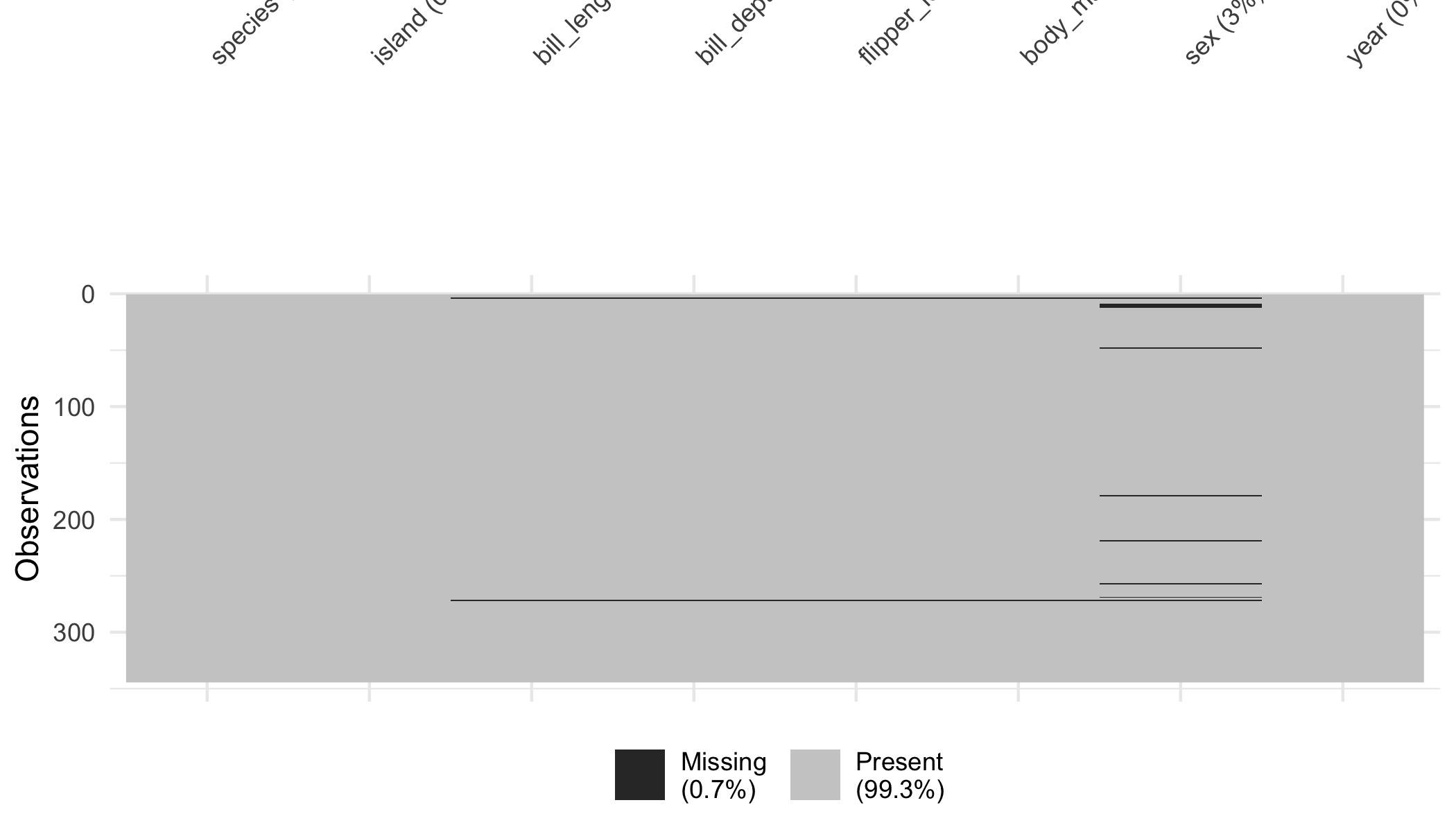
sex, with two rows missing all four morphology measurements.
Everything should be made as simple as possible, but not simpler.
Albert Einstein, attributed (1933)
Adapted from author’s lecture notes and supporting materials for a graduate practicum in biostatistics.
Answer the following questions to see if you can bypass this chapter. You can find the answers at the end of the chapter in Section 30.18.
palmerpenguins::penguins dataset contain, and how should they be handled?body_mass_g on flipper_length_mm, what is the first diagnostic plot you should produce before interpreting any coefficient?By the end of this chapter you should be able to:
zzcollab.zztable1.The Palmer Penguins dataset (Horst et al., 2022) is the successor to iris. It has enough structure to illustrate the full arc of an analysis, from wrangling through descriptives and inference to reporting, and it does so without the colonial baggage that accompanies Fisher’s irises. We shall work it end to end here, as a template for the analyses that follow.
A teaching dataset carries one hazard worth naming before we start. Penguins is clean, and clean data invite the habit of skipping the steps this book has spent twenty chapters arguing for. The reasonable-sounding excuse is that nothing here needs them. That is the wrong lesson to take from a worked example. The point of running the full arc on an easy dataset is that the arc is what you practice, so that it is already automatic when the data are difficult and the stakes are real. Every step below is performed deliberately, including the ones that look unnecessary, and the chapter says why each is performed rather than assuming it is obvious.
The dataset is small enough that the analysis runs in seconds, but rich enough to exercise every component of the workflow this Practicum has built. By the end of this chapter you should have a complete, deposited, citable compendium that demonstrates the practices of Parts I through VI. The obligations that attach to it once it exists, how it is deposited and what it may still get wrong, are taken up in Part VIII.
Even on a small clean dataset, judgment applies.
Document the cleaning decisions. Eleven rows have at least one missing value. Dropping them or imputing changes the analysis; the choice should be deliberate and documented. The ‘palmerpenguins is so clean it doesn’t matter’ attitude leads to bad habits on dirtier data.
Pick the encoding deliberately. Species is the most natural stratification; island and sex are secondary. The species reference level matters for coefficient interpretation; pick it to match the substantive question (is one species the reference baseline, or do you want contrasts among all three?).
Resist over-modeling. A simple linear model of body mass on flipper length adjusted for species fits the data well; an interaction model adds parameters with limited gain. Picking the simpler model and reporting an AIC comparison is more defensible than picking the more elaborate one because it has more p-values.
Treat the case study as a template. The arc here (scaffold → clean → describe → visualize → fit → diagnose → report → deposit) is what every project should follow. Practicing on penguins is practicing for every future project.
These judgments scale to substantive analyses; penguins is the small example where they are easy to articulate.
palmerpenguins::penguins contains 344 observations of three penguin species (Adelie, Chinstrap, Gentoo) collected at three islands (Biscoe, Dream, Torgersen) in the Palmer Archipelago of Antarctica during 2007–2009.
Variables:
species: Adelie, Chinstrap, Gentoo (3 levels).island: Biscoe, Dream, Torgersen.bill_length_mm: continuous.bill_depth_mm: continuous.flipper_length_mm: continuous, the strongest predictor of body mass.body_mass_g: continuous, the analytic outcome.sex: Male, Female (with 11 missing).year: 2007, 2008, or 2009.The dataset has a near-balanced design: each species appears at one or two islands. Adelies appear at all three islands; Chinstraps only at Dream; Gentoos only at Biscoe. This means species and island are not separable in the full model; choosing species as the stratification puts island in the role of an additional confounder rather than an independent factor.
mkdir penguins-analysis
cd penguins-analysis
zzc analysis             # tidyverse + palmerpenguins profile
make r                   # enter the container
zzc analysis produces the Five Pillars (Chapter 13): Dockerfile, renv.lock, .Rprofile, source-code directories, and a README pointing at the data. make r builds the image (slow on first run; cached subsequently) and drops you into an R session inside the container.
Verify the compendium is well-formed:
zzrenvcheck::check_packages()This audits all five Pillars and produces a list of any inconsistencies. For a fresh zzc project, the output should be clean.
library(palmerpenguins)
library(naniar)

# inspect missingness
vis_miss(penguins)sex, with two rows missing all four morphology measurements.
miss_var_summary(penguins)
#> # A tibble: 8 × 3
#>   variable          n_miss pct_miss
#>   <chr>              <int>    <num>
#> 1 sex                   11    3.20
#> 2 bill_length_mm         2    0.581
#> 3 bill_depth_mm          2    0.581
#> 4 flipper_length_mm      2    0.581
#> 5 body_mass_g            2    0.581
#> 6 species                0    0
#> 7 island                 0    0
#> 8 year                   0    0
Missingness is mostly in sex (11 rows, 3.2%); two rows are missing all four morphology measurements (likely lost CRFs from the same penguin).
For this case study, complete-case is the appropriate strategy: the missing fraction is small, MAR-on-other-variables is plausible (missingness probably reflects field-data collection issues, not a relationship to body mass), and the analysis is descriptive rather than inferential. Document the choice:
We drop 11 rows; analyses use \(n = 333\).
library(zztable1)

zztable1::table1(
  bill_length_mm + bill_depth_mm + flipper_length_mm +
    body_mass_g + sex ~ species,
  data    = penguins_clean,
  totals  = TRUE,
  layout  = 'latex'
) |>
  zzobj2fig::o2f(filename = 'table1', sub_dir = 'figures')
The produced Table 1 has columns for each species plus an overall column, and rows for each variable. Continuous variables show mean (SD); categorical variables show n (%).
Formatting notes: zztable1 uses three significant digits for continuous summaries, no row p-values by default (Table 1 is descriptive, not inferential), and ordering the species columns by the natural taxonomic order rather than alphabetical.
library(ggplot2)

theme_set(theme_minimal())

ggplot(penguins_clean,
       aes(flipper_length_mm, body_mass_g, color = species)) +
  geom_point(alpha = 0.7) +
  scale_color_brewer(palette = "Dark2") +
  labs(x = "Flipper length (mm)",
       y = "Body mass (g)",
       color = "Species") +
  facet_wrap(~ island)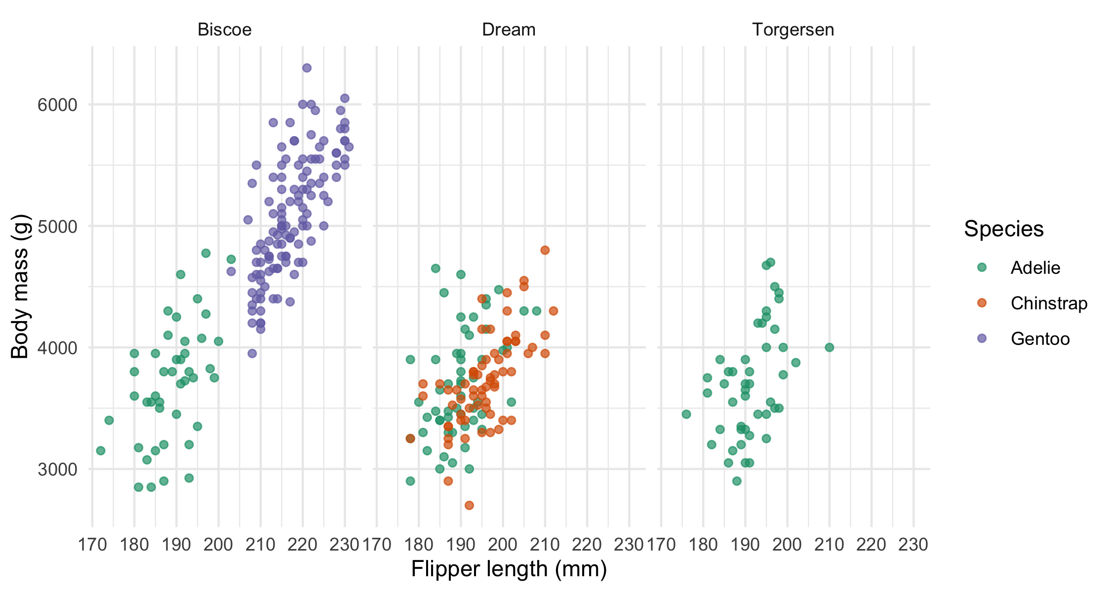
What the plot reveals:
The first plot is exploratory: identify the structure before the model. The structure suggests the model: species as a categorical predictor, flipper length as a continuous predictor.
fit <- lm(body_mass_g ~ flipper_length_mm + species,
          data = penguins_clean)
broom::tidy(fit, conf.int = TRUE)
#> # A tibble: 4 × 7
#>   term              estimate std.error statistic  p.value conf.low conf.high
#>   <chr>                <dbl>     <dbl>     <dbl>    <dbl>    <dbl>     <dbl>
#> 1 (Intercept)        -4013.     586.       -6.85 3.74e-11  -5166.    -2860.
#> 2 flipper_length_mm     40.6      3.08     13.2  3.64e-32     34.5      46.7
#> 3 speciesChinstrap    -205.      57.6      -3.57 4.14e- 4   -319.      -92.1
#> 4 speciesGentoo 285. 95.4 2.98 3.08e- 3 96.8 472.Every number in the paragraph that follows is computed by the chunk above rather than typed in, which is the discipline of Chapter 15 applied to the book’s own case study.
The intercept is the predicted body mass of an Adelie penguin at a flipper length of zero. It is an extrapolation far outside the data and is not interpretable as anything; it exists to anchor the line. The flipper_length_mm coefficient is the within-species slope: the expected difference in body mass between two penguins of the same species whose flipper lengths differ by one millimeter.
The species coefficients deserve more care, because they are the place a reader is most likely to misread the table. They are differences from Adelie at the same flipper length, and that is not the same quantity as the difference in average mass between the species. Gentoos average roughly 1,390 g heavier than Adelies in this dataset. The speciesGentoo coefficient is a small fraction of that, because Gentoos also have much longer flippers, and the model has already credited the flipper-length term with most of the difference. The adjusted coefficient answers ‘how much heavier is a Gentoo than an Adelie with the same flippers’, which is a narrower and more surprising question than the one a reader assumes it answers. Reporting the adjusted coefficient as though it were the species difference is the single easiest error to make with this table.
The \(R^2\) from glance() is respectable but not overwhelming, and it is worth saying plainly that a respectable \(R^2\) on a clean morphometric dataset is not evidence that the model is well specified. It says the predictors and the outcome are related, and nothing about whether the functional form is right. That is what the diagnostics are for.
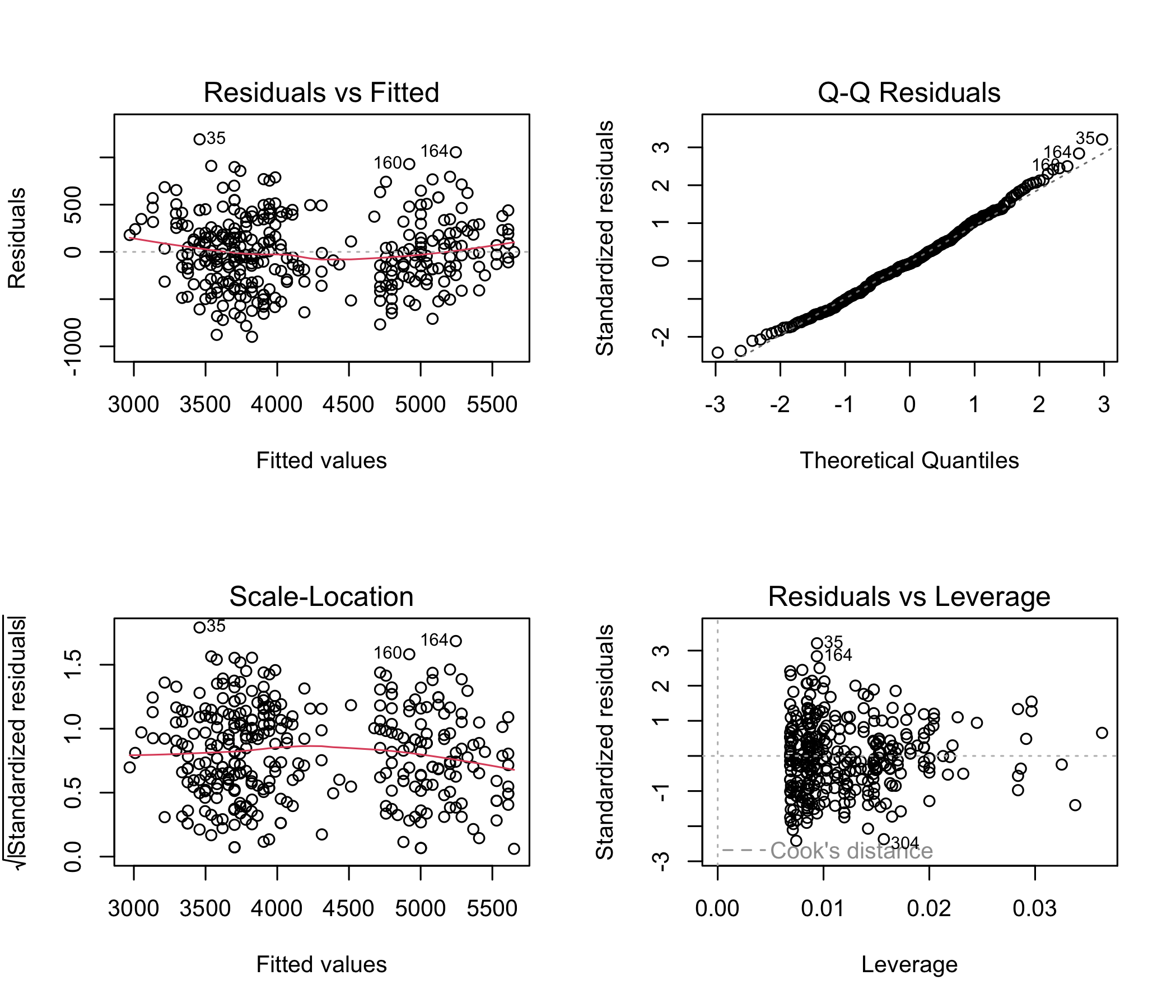
lm diagnostic plots for the fitted model. Residuals versus fitted and scale-location test the mean and variance structure; the Q-Q plot tests the residual distribution; residuals versus leverage identifies influential observations.
The four diagnostic plots:
For penguins, the diagnostics are clean. For real clinical data, the diagnostics rarely look this good; the discipline is to check, then remedy.
The compendium’s analysis/paper/paper.qmd:
---
title: "Palmer Penguins: a case study"
format:
html: default
pdf: default
execute:
echo: false
freeze: auto
---
```r
#| include: false
library(palmerpenguins)
library(tidyverse)
library(broom)
penguins_clean <- na.omit(penguins)
fit <- lm(body_mass_g ~ flipper_length_mm + species,
data = penguins_clean)
```
# Methods
We analyzed the `palmerpenguins` dataset
[@horst2022palmerpenguins], $n = `{r} nrow(penguins_clean)`$
after dropping $`{r} sum(!complete.cases(penguins))`$
rows with missing values. Body mass was modeled
as a function of flipper length and species via
ordinary least squares.
# Results
@fig-scatter shows the relationship; @tbl-coef
gives the fitted coefficients.
```r
#| label: fig-scatter
#| fig-cap: "Body mass vs. flipper length, by species"
ggplot(penguins_clean,
aes(flipper_length_mm, body_mass_g, color = species)) +
geom_point(alpha = 0.7)
```
```r
#| label: tbl-coef
#| tbl-cap: "Fitted regression coefficients"
broom::tidy(fit, conf.int = TRUE)
```make render inside the container reproduces the paper from raw data to typeset output. The render uses the cached _freeze/ directory for the expensive computation; subsequent renders are fast.
# tag the release
git tag -a v1.0 -m "Penguins case study, complete"
git push origin v1.0

# Zenodo + GitHub integration produces a DOI from the tag
# (configure once at zenodo.org/account/settings/github)
The deposited artifact is the GitHub repo at the tagged commit, with a Zenodo DOI. The README explains:
docker build && docker run).palmerpenguins).A reader, given the DOI, can rebuild the paper in two commands. That is what reproducible research looks like.
LLMs handle this kind of clean dataset well; the trap is over-modeling.
Prompt 1: suggesting plots. Paste the data dictionary and ask: ‘suggest three plots that would reveal interesting structure.’
What to watch for. The LLM should propose plots motivated by the variables (the bivariate flipper-mass scatter, marginal mass distributions by species, bill morphology scatter). Generic templates (‘a histogram of each variable’) are less useful.
Verification. Render each suggested plot; keep the ones that show structure not visible in the others.
Prompt 2: imputation. Ask: ‘how should I handle the 11 rows with missing sex?’
What to watch for. Three reasonable answers: complete-case (if you do not need sex), single imputation from sex-specific distributions, or formal MICE. The LLM should state the trade-offs; if it picks one unreservedly, push for the alternatives.
Verification. Run the analysis under complete-case and under MICE; compare results. For penguins the difference is small.
Prompt 3: writing results. Paste the fitted regression and ask the LLM to write the results paragraph.
What to watch for. Reference level (Adelie, not ‘penguins of unspecified species’). CIs rather than p-values. No overclaiming.
Verification. Have a colleague read the paragraph and underline anything they would flag in peer review.
The case study is a template, and three habits are what it is a template for:
zzc analysis before any analysis code. The discipline is non-negotiable.body_mass_g ~ flipper_length_mm * species. Test the interaction; report AIC against the main-effects model.species on the four morphometric measurements, and report how often it recovers the observed species.On your own machine. No answer key; these are things you do to a repository, not to data.
make render and verify the outputs match the ones checked into the reference repository.palmerpenguins package vignettes at allisonhorst.github.io/palmerpenguins, teaching examples.palmerpenguins::penguins contains 11 rows with at least one missing value (most commonly sex). The appropriate handling is first to document the missing pattern (naniar::vis_miss()), then to choose a strategy before analysis: complete-case if the missingness is MCAR and the fraction is small; imputation if more than ~5% of rows are affected or if missingness is informative.zzcollab compendium with the analysis profile: mkdir penguins && cd penguins && zzc analysis produces the Five Pillars (Chapter 13). The command completes in under a minute and the resulting directory renders out of the box.