library(naniar)
library(palmerpenguins)

vis_miss(penguins)               # row-by-column heatmap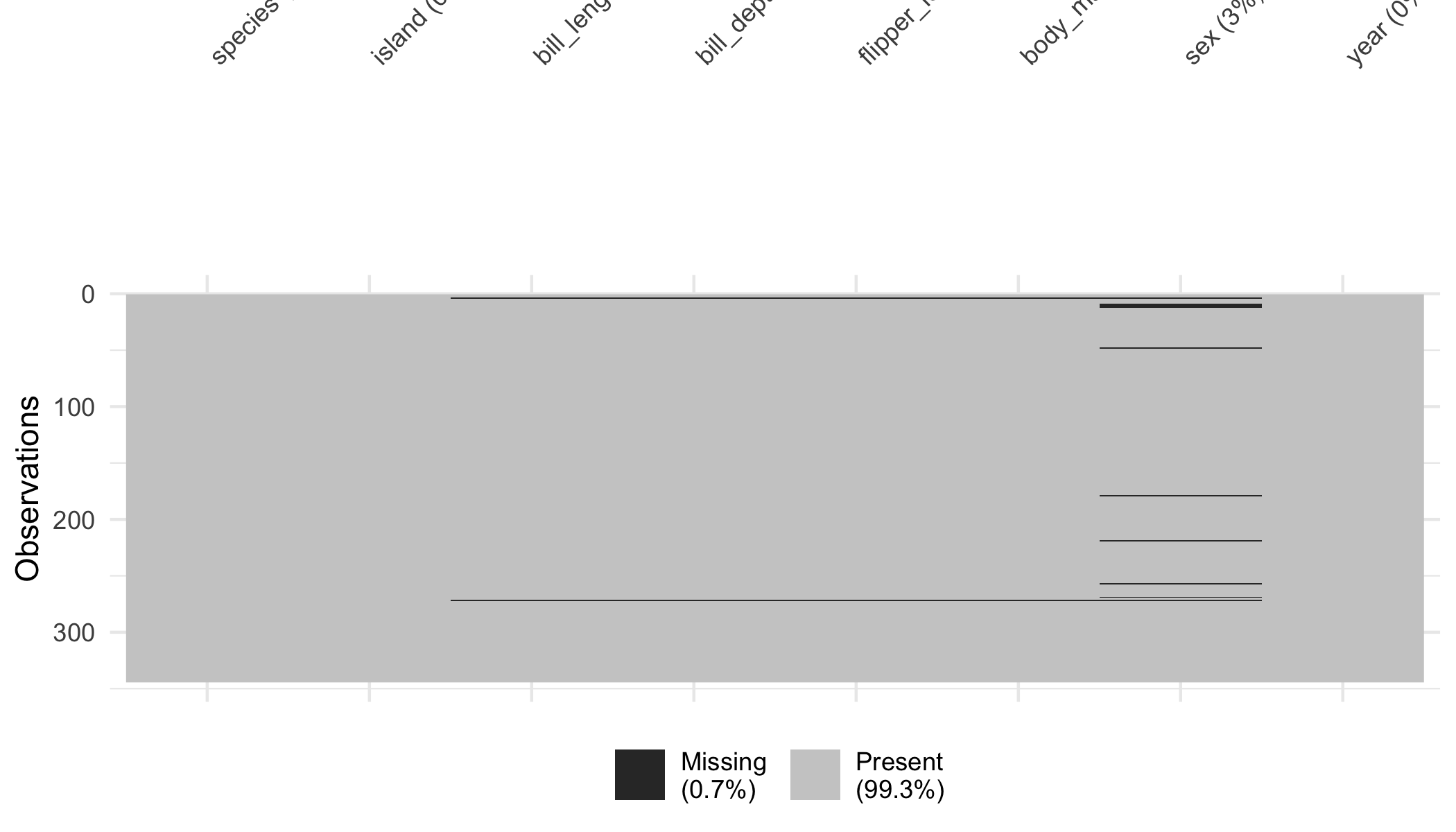
sex variable carries most of the missingness.
Absence of evidence is not evidence of absence.
Douglas G. Altman and J. Martin Bland, British Medical Journal (1995)
The survey of peer US biostatistics MS programs (Appendix B) found missing-data handling taught as a core or near-core topic at a majority of them, including dedicated courses at Michigan (University of Michigan School of Public Health, 2024) and the University of Washington (Sadinle, 2019), and coverage within the curricula at Emory (Emory University Rollins School of Public Health, 2024), Yale (Yale School of Public Health, 2024), Iowa (University of Iowa College of Public Health, 2024), UT Health Houston (UT Health Houston School of Public Health, 2024), and Florida (University of Florida College of Public Health and Health Professions, 2025). Every real clinical dataset has missing values, and the decisions around them often move point estimates more than the model choice does. This chapter is the Practicum’s response.
Answer the following questions to see if you can bypass this chapter. You can find the answers at the end of the chapter in Section 23.19.
By the end of this chapter you should be able to:
naniar::vis_miss() and naniar::gg_miss_var().mice using predictive mean matching for continuous variables and logistic regression for binary variables.Missing data is, perhaps, the least-loved topic in an MS curriculum, and the reason is that its answers are rarely clean. Complete-case analysis is simple, but it throws information away and biases estimates under anything stronger than MCAR. Multiple imputation preserves the information, but it adds a modeling layer with assumptions of its own. Sensitivity analysis is essential, but it is open-ended. There is, in short, no method here that is free of difficulty.
The pragmatic stance, in our view, is this: document the missingness, be honest about the mechanism, implement one principled approach (most often multiple imputation via mice), and report the sensitivity of conclusions to alternative approaches.
Missing data is the chapter where judgment matters most.
The mechanism is an assumption, not a fact. MCAR/MAR/MNAR cannot be distinguished from the observed data alone. Whatever mechanism you assume is a substantive claim about why the missingness occurred, defended by what you know about the data collection. ‘The patient was lost to follow-up’ could be MCAR (random administrative loss), MAR (loss correlated with observed baseline), or MNAR (loss correlated with the unobserved outcome). The correct response is to argue from the clinical context, not from a hypothesis test.
Imputation is modeling. When you impute, you are fitting a model for the missing values. That model has assumptions. Bad imputation introduces bias more cleanly than complete-case analysis would. The tools (mice, Amelia, mi) make imputation easy; making it correct requires attending to the imputation model’s specification.
Outcome and predictor missingness are not symmetric. Missing outcome data with MAR-on- covariates is well-handled by likelihood methods. Missing predictor data is trickier and almost always demands imputation. The two cases warrant different strategies.
Pre-specify the missing-data plan. The SAP (Chapter 24) should specify the primary missing-data approach before data access. Choosing the strategy after seeing the data – ‘we tried complete case, then MI, and report MI because it gave a smaller p-value’ – is indistinguishable from p-hacking.
These judgments are what make missing-data handling defensible rather than mechanical.
Rubin (1976) defines three missingness mechanisms. Let \(Y\) be the variable of interest; \(R\) the indicator that \(Y\) is observed; \(X\) other observed variables.
MCAR (Missing Completely At Random). \(P(R \mid Y, X) = P(R)\): missingness is independent of both observed and unobserved data. Example: a clinical CRF page is occasionally lost in the mail, with the loss process unrelated to patient or measurement.
MAR (Missing At Random). \(P(R \mid Y, X) = P(R \mid X)\): missingness depends only on observed data. Example: older patients more often miss follow-up visits than younger ones; conditional on age, missingness is independent of the missing outcome.
MNAR (Missing Not At Random). \(P(R \mid Y, X)\) depends on \(Y\) itself, even after conditioning on \(X\). Example: patients with worse symptoms are more likely to drop out because they get worse, and the dropout itself is the bad news. Conditional on observed covariates, missingness still depends on the unobserved outcome.
The three are progressively more restrictive in the methods they allow:
| Mechanism | Complete case | Likelihood / MI | Sensitivity needed? |
|---|---|---|---|
| MCAR | Unbiased | Unbiased | No |
| MAR | Biased | Unbiased | No |
| MNAR | Biased | Biased | Yes |
In practice, MCAR is rare, MAR is the default working assumption, and MNAR is what sensitivity analyses are for. The data cannot distinguish MAR from MNAR, so the choice rests on substantive reasoning.
One case that recurs in biomarker work does not fit this taxonomy comfortably, and it is worth naming because the reflex it invites is wrong. An assay reports a concentration only above its limit of detection; below that, the instrument returns not a value but the information that the value is small. This is left censoring rather than missingness. The distinction matters because the data are not absent: knowing a concentration lies below a known threshold is considerably more than knowing nothing, and an analysis that discards those observations, or that substitutes a constant such as the limit divided by the square root of two, throws away information and distorts the variance in ways multiple imputation under MAR will not repair. The methods that suit this case are its own family: regression on order statistics, censored maximum likelihood, and multiple imputation adapted for a censoring threshold. The in-house zzmesoimpute package provides a common interface across them for multiplexed immunoassay data, which is the setting where the problem is most often met. The general lesson generalizes past the package: before choosing a missing-data method, establish whether the values are missing or merely unobserved below a bound, because those are different problems with different remedies.
Before any imputation, look at the pattern. The naniar package provides ggplot-friendly diagnostics. The row-by-column heatmap is the first thing to look at: it shows at a glance which variables carry missingness and whether it clusters in particular rows.
library(naniar)
library(palmerpenguins)
vis_miss(penguins) # row-by-column heatmapsex variable carries most of the missingness.
A per-variable bar chart quantifies what the heatmap suggests:
gg_miss_var(penguins) # bar chart of missing per variable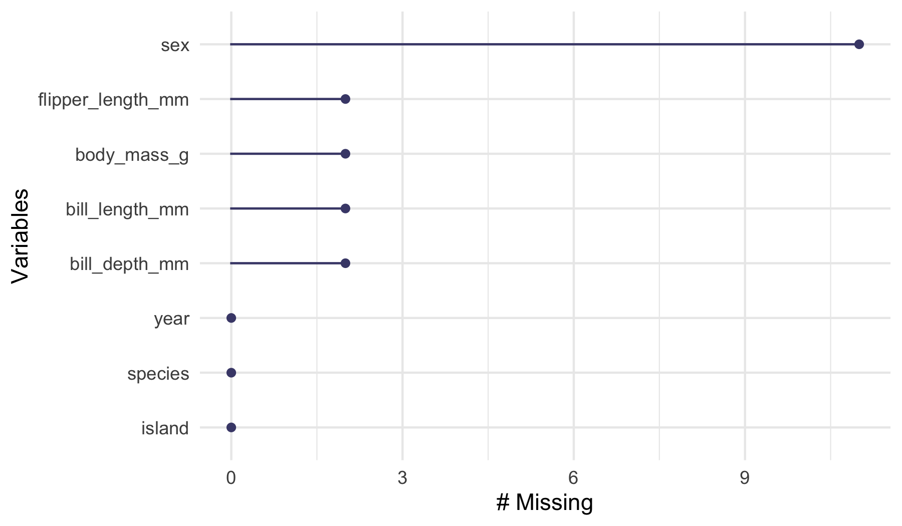
sex account for essentially all the missingness in the penguin data.
Two further diagnostics are worth knowing. The UpSet plot shows how missingness co-occurs across variables, and the case summary counts missing cells per row:
gg_miss_upset(penguins) # UpSet-style intersection plot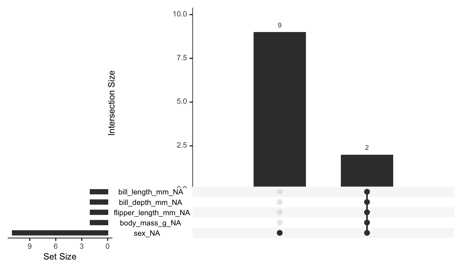
sex from the two rows missing every morphology measurement.
miss_case_summary(penguins)      # how many missing per row
#> # A tibble: 344 × 3
#>     case n_miss pct_miss
#>    <int>  <int>    <dbl>
#>  1     4      5     62.5
#>  2   272      5     62.5
#>  3     9      1     12.5
#>  4    10      1     12.5
#>  5    11      1     12.5
#>  6    12      1     12.5
#>  7    48      1     12.5
#>  8   179      1     12.5
#>  9   219      1     12.5
#> 10   257      1     12.5
#> # ℹ 334 more rows
Patterns to look for:
The pattern affects strategy. Monotone missingness admits simpler imputation models (sequential regression). Arbitrary missingness needs the full multivariate machinery (mice with chained equations).
The simplest approach: drop rows with any missingness. R’s default for lm, glm, and most modeling functions is na.omit (or na.action = na.omit).
When complete-case is acceptable:
When complete-case is not acceptable: substantial missingness with plausible MAR. The bias can be large.
Mean imputation replaces missing values with the sample mean. Two problems:
Last observation carried forward (LOCF) is deprecated except as a pre-specified sensitivity analysis. It assumes patients who drop out remain at their last observed value, which is biologically implausible for most diseases. The ICH E9(R1) addendum (International Council for Harmonisation, 2019) explicitly cautions against it, and Harrell’s author checklist (Harrell, 2024) rules it out without the sensitivity-analysis exemption, on the grounds that an assumption no one believes is not made believable by being labeled.
Single regression imputation without noise produces coefficients that are too tight: the imputed values lie exactly on a regression surface, hiding the variability that should be present.
The common theme: single imputation underestimates variance because it pretends the imputed values have no uncertainty. Multiple imputation fixes this by drawing many plausible values per missing cell.
mice
Multiple imputation proceeds in three steps, shown in Figure 23.4: impute several completed datasets, analyze each one separately, then pool the results. The reason for the fan-out and recombination is the whole point of the method: the variation between the \(M\) analyses is what carries the uncertainty due to missingness that single imputation discards.
flowchart TD
  D["Incomplete<br/>data"] --> S1["Set 1"]
  D --> S2["Set 2"]
  D --> Sm["Set M"]
  S1 --> F1["Fit 1"]
  S2 --> F2["Fit 2"]
  Sm --> Fm["Fit M"]
  F1 --> P["Pool<br/>Rubin's rules<br/><i>within + between variance</i>"]
  F2 --> P
  Fm --> P
  P --> R["One pooled<br/>estimate and SE"]
The three steps in detail:
In R:
library(mice)

# step 1: impute
imp <- mice(airquality, m = 25, method = "pmm", seed = 1,
            printFlag = FALSE)

# step 2: analyze each
fits <- with(imp, lm(Ozone ~ Solar.R + Wind + Temp))

# step 3: pool
pooled <- pool(fits)
summary(pooled, conf.int = TRUE)
#>          term     estimate  std.error statistic       df      p.value
#> 1 (Intercept) -63.99524051 23.6467109 -2.706306 74.34229 8.433947e-03
#> 2     Solar.R   0.05730006  0.0233814  2.450668 91.64428 1.615709e-02
#> 3        Wind  -3.03601187  0.6767108 -4.486424 75.46241 2.550252e-05
#> 4        Temp   1.61531187  0.2496912  6.469237 91.43913 4.779282e-09
#>           2.5 %     97.5 %      conf.low  conf.high
#> 1 -111.10873627 -16.881745 -111.10873627 -16.881745
#> 2    0.01086017   0.103740    0.01086017   0.103740
#> 3   -4.38395356  -1.688070   -4.38395356  -1.688070
#> 4    1.11936297   2.111261    1.11936297   2.111261
mice defaults:
method = "pmm" for continuous variables: predictive mean matching. The imputed value is drawn from the observed values whose predicted values are closest to the missing observation’s predicted value. PMM is robust to model misspecification.method = "logreg" for binary, polyreg for unordered categorical, polr for ordered categorical. mice picks defaults appropriately.m = 5 is the historical default; m = 25 or higher is the modern recommendation (Bodner, 2008): \(M\) should exceed the percentage of missing information.seed: set for reproducibility.Always include the outcome in the imputation model when imputing predictors: omitting it biases the imputation toward the null (Moons et al., 2006).
Pool the \(M\) analyses:
The \((1 + 1/M)\) factor is a finite-sample correction.
Degrees of freedom use the Barnard-Rubin adjustment (the mice default), which produces slightly conservative t-tests for moderate \(M\).
mice::pool() does all of this automatically. Inspect the components:
fmi (fraction of missing information) is a useful summary: how much of the variance in \(\hat\beta\) is due to missing data. Values above 0.5 suggest the analysis is heavily influenced by imputation; consider sensitivity.
Using airquality:
library(naniar)
library(mice)
library(broom.mixed)

# 1. visualize pattern
vis_miss(airquality)
gg_miss_upset(airquality)

# 2. complete-case
fit_cc <- lm(Ozone ~ Solar.R + Wind + Temp, data = airquality)
broom::tidy(fit_cc, conf.int = TRUE)
nrow(fit_cc$model)              # 111 rows used

# 3. multiple imputation
imp <- mice(airquality, m = 25, method = "pmm", seed = 1,
            printFlag = FALSE)
fits <- with(imp, lm(Ozone ~ Solar.R + Wind + Temp))
pooled <- pool(fits)
summary(pooled, conf.int = TRUE)
nrow(airquality)                # 153 rows analyzed via MI

# 4. sensitivity: delta adjustment
# (assume Ozone with missingness is systematically
# 0.5 SD lower than MAR-imputed values)
imp_delta <- mice(airquality, m = 25, method = "pmm",
                  seed = 1, printFlag = FALSE)
imp_delta$imp$Ozone <- imp_delta$imp$Ozone -
                       0.5 * sd(airquality$Ozone, na.rm = TRUE)
fits_delta <- with(imp_delta, lm(Ozone ~ Solar.R + Wind + Temp))
pool(fits_delta) |> summary()
Compare the three coefficient estimates and their standard errors. If the conclusions are similar under all three, you have a robust result. If they diverge, the missing-data assumption is load-bearing and the paper should say so.
CONSORT 2010 (item 13b, randomized trials) (Schulz et al., 2010) and STROBE (item 12c, observational studies) (Elm et al., 2007) require:
A sample reporting paragraph:
Of 1,000 enrolled patients, 23 (2.3%) had missing baseline body mass index and 47 (4.7%) had missing 12-month follow-up outcome. Patterns of missingness are shown in Supplementary Figure S1. Missing baseline BMI was assumed missing at random (MAR) given age, sex, and treatment arm. Missing follow-up outcomes were imputed using multiple imputation with chained equations (\(M = 25\), predictive mean matching for continuous variables, logistic regression for binary), including all baseline covariates and the treatment indicator. Pooled estimates use Rubin’s rules. Sensitivity to MNAR was assessed via a delta adjustment of \(\pm 0.5\) SD on the imputed outcomes; results were qualitatively similar (Supplementary Table S5).
The level of detail demonstrates that you have thought about the issue, not papered over it.
CONSORT and STROBE set the floor. Harrell’s author checklist (Harrell, 2024), written from the reviewer’s side of the exchange, adds an item the reporting standards leave implicit: an incomplete record is not a disposable one. Dropping every patient with any missing covariate is a decision with consequences for both power and bias, and it requires the same justification in the methods section as an imputation model would. If the complete-case sample differs from the enrolled sample in ways the reader can check, show the comparison; if it does not differ on anything you measured, say so, and say what you could not measure.
Three standard sensitivity approaches:
Delta adjustment. After MI under MAR, shift the imputed values by \(\pm \delta\) to mimic an MNAR scenario. Refit the analysis. The result shows how robust conclusions are to the MNAR direction. Implementation: edit imp$imp after calling mice, then re-fit.
Tipping-point analysis. Vary \(\delta\) continuously and find the value at which the conclusion ‘tips’ (e.g., the treatment effect loses statistical significance). The tipping point’s clinical plausibility is the question: if it requires a \(\delta\) much larger than clinical experience suggests is realistic, the conclusion is robust.
Pattern-mixture models. Specify different imputation models for different missingness patterns. The framework is explicit about MNAR assumptions per pattern; the implementation is more involved than delta adjustment.
For a typical paper, delta adjustment with one or two values of \(\delta\) is sufficient sensitivity. For high-stakes regulatory submissions or papers where the missingness is large, tipping-point analysis is more thorough.
The SAP (Chapter 24) should specify the primary missing-data strategy before data access. A typical pre-specification:
Primary analysis will use multiple imputation with \(M = 25\) datasets, predictive mean matching for continuous variables and logistic regression for binary variables, including all outcome and covariate information. Pooling follows Rubin’s rules. Sensitivity to the MAR assumption will be assessed via a delta adjustment of \(\pm 0.5\) SD on the imputed outcome.
Specifying details (\(M\), methods, sensitivity) prevents the post-hoc choice that turns missingness handling into another researcher degree of freedom.
LLMs handle the mechanics; the substantive mechanism reasoning is the analyst’s.
Prompt 1: classifying the mechanism. Paste a missingness summary and a brief description of the data collection; ask: ‘classify each variable’s likely mechanism (MCAR / MAR / MNAR) and justify.’
What to watch for. The LLM may overreach: it cannot know the substantive context, so its classifications are guesses. Treat the output as a starting list, not an answer. Add the clinical reasoning yourself.
Verification. Discuss with the clinical collaborator. Their substantive view wins; update the classifications accordingly.
Prompt 2: writing the mice call. Describe the dataset (variable types, missingness rates) and ask: ‘write the mice call with appropriate methods per variable and an explanation of the choices.’
What to watch for. Method selection per variable type. Inclusion of the outcome in the predictor matrix. Use of m = 25 or higher rather than the historical m = 5. The LLM should know all of this; if it does not, push.
Verification. Run the call. Inspect imp$method; verify each variable has the expected method. Check imp$predictorMatrix; verify the outcome is included for predictor imputation.
Prompt 3: writing the SAP missing-data section. Describe the trial and ask the LLM to draft the missing-data subsection of the SAP.
What to watch for. The pre-specification should be specific enough that a reader cannot ask ‘which?’ on key choices. Vague language (‘appropriate imputation’) is not pre-specification. The LLM may be vague; push for specifics.
Verification. Show to a colleague who has seen FDA or EMA SAPs; their feedback recalibrates.
Three habits keep missing data a stated assumption rather than a silent one:
airquality (built-in). Visualize the missingness pattern with naniar. Fit lm(Ozone ~ Solar.R + Wind + Temp) via complete-case analysis; then via multiple imputation with m = 20. Compare coefficients and standard errors.mice::ampute() function to induce MAR missingness on a complete dataset. Fit the analysis on the full data and on the amputed-then-imputed data. Compare estimates; verify MI recovers the truth approximately.Writing, not computing. No answer key; this is a document, and what a good one establishes is stated rather than computed.
1. Complete case against multiple imputation.
cc <- lm(Ozone ~ Solar.R + Wind + Temp, data = airquality)

imp20 <- mice(airquality, m = 20, method = "pmm",
              seed = 2, printFlag = FALSE)
mi <- pool(with(imp20, lm(Ozone ~ Solar.R + Wind + Temp)))

comparison <- dplyr::bind_rows(
  broom::tidy(cc) |> dplyr::mutate(method = "complete case"),
  summary(mi) |>
    tibble::as_tibble() |>
    dplyr::rename(term = term, estimate = estimate,
                  std.error = std.error) |>
    dplyr::mutate(method = "multiple imputation")
) |>
  dplyr::select(method, term, estimate, std.error)

comparison
#> # A tibble: 8 × 4
#>   method              term        estimate std.error
#>   <chr>               <chr>          <dbl>     <dbl>
#> 1 complete case       (Intercept) -64.3      23.1
#> 2 complete case       Solar.R       0.0598    0.0232
#> 3 complete case       Wind         -3.33      0.654
#> 4 complete case       Temp          1.65      0.254
#> 5 multiple imputation (Intercept) -62.1      22.2
#> 6 multiple imputation Solar.R       0.0605    0.0221
#> 7 multiple imputation Wind         -3.12      0.640
#> 8 multiple imputation Temp          1.59      0.243
The coefficients move little; the standard errors are what change, and they change in both directions. MI uses all 153 rows rather than the 111 complete ones, which tightens some estimates, while the between-imputation variance widens others. A method that only ever tightened intervals would be recovering information it does not have.
2. Bias of three methods under MAR.
set.seed(11)

one_rep <- function(n = 200, beta = 1) {
  x <- rnorm(n); z <- rnorm(n)
  y <- beta * x + 0.5 * z + rnorm(n)
  # MAR: x goes missing more often when z is large
  x[runif(n) < plogis(-1.4 + z)] <- NA
  d <- data.frame(y, x, z)

  b_cc <- coef(lm(y ~ x + z, data = d))[["x"]]

  d_mean <- d
  d_mean$x[is.na(d_mean$x)] <- mean(d_mean$x, na.rm = TRUE)
  b_mean <- coef(lm(y ~ x + z, data = d_mean))[["x"]]

  im <- mice(d, m = 5, printFlag = FALSE, seed = 1)
  s_mi <- summary(pool(with(im, lm(y ~ x + z))))
  s_mi <- s_mi[s_mi$term == "x", ]

  c(cc = b_cc - beta,
    mean = b_mean - beta,
    mi = s_mi$estimate - beta,
    se_cc = summary(lm(y ~ x + z, data = d))$coefficients["x", 2],
    se_mean = summary(lm(y ~ x + z,
                         data = d_mean))$coefficients["x", 2],
    se_mi = s_mi$std.error)
}

# 100 replicates rather than 500, to keep the book's build fast
res <- rowMeans(replicate(100, one_rep()))
round(res, 3)
#>      cc    mean      mi   se_cc se_mean   se_mi
#>   0.021   0.021   0.026   0.079   0.091   0.073
Read the two halves separately. All three methods are close to unbiased in the coefficient, because the missingness depends on z and z is in the model, which is what MAR means. The bias column is not where mean imputation fails.
The standard errors separate the three, and not in the direction the usual slogan suggests. Multiple imputation is tightest, complete case wider, and mean imputation widest of all.
The ordering is worth sitting with, because the textbook warning about mean imputation is that it understates uncertainty, and that is not what happens here. Two different quantities are being confused. Mean imputation does shrink the spread of the variable it fills, which the antipattern earlier in this chapter demonstrates directly. But the standard error of a regression coefficient is not that spread: filling 20% of a covariate with a constant destroys the covariance between x and y in those rows, which weakens the estimated relationship and inflates the residual variance. The reported error goes up, not down.
The variance-understatement warning applies where the naive error ignores the imputation step, most sharply when the outcome itself is filled in. Here MI wins on the honest grounds: it uses all 200 rows rather than the roughly 160 complete ones, and it carries the between-imputation variance forward rather than pretending the filled values were observed.
4. Ampute, impute, and check recovery.
set.seed(12)
complete_data <- na.omit(airquality[, c("Ozone", "Solar.R",
                                        "Wind", "Temp")])

truth <- coef(lm(Ozone ~ Solar.R + Wind + Temp,
                 data = complete_data))

amputed <- mice::ampute(complete_data, prop = 0.3,
                        mech = "MAR")$amp
recovered <- summary(pool(with(
  mice(amputed, m = 20, printFlag = FALSE, seed = 3),
  lm(Ozone ~ Solar.R + Wind + Temp))))

data.frame(term = names(truth),
           truth = round(unname(truth), 3),
           recovered = round(recovered$estimate, 3))
#>          term   truth recovered
#> 1 (Intercept) -64.342   -59.119
#> 2     Solar.R   0.060     0.060
#> 3        Wind  -3.334    -3.178
#> 4        Temp   1.652     1.548
MI recovers the full-data coefficients approximately, which is the claim being checked. ‘Approximately’ is doing real work: a single run can miss by more than you expect, and one replicate is a demonstration rather than evidence.
5. Delta adjustment and the tipping point.
set.seed(13)
n <- 400
d <- data.frame(x = rnorm(n))
d$y <- rbinom(n, 1, plogis(0.4 * d$x))
d$x[runif(n) < 0.25] <- NA

delta_fit <- function(delta) {
  im <- mice(d, m = 10, printFlag = FALSE, seed = 4)
  im$imp$x <- im$imp$x + delta
  s <- summary(pool(with(im, glm(y ~ x, family = binomial))))
  s$estimate[s$term == "x"]
}

deltas <- seq(-1, 1, by = 0.25)
curve <- data.frame(delta = deltas,
                    estimate = vapply(deltas, delta_fit, numeric(1)))

ggplot2::ggplot(curve, ggplot2::aes(delta, estimate)) +
  ggplot2::geom_line() +
  ggplot2::geom_hline(yintercept = 0, linetype = 2)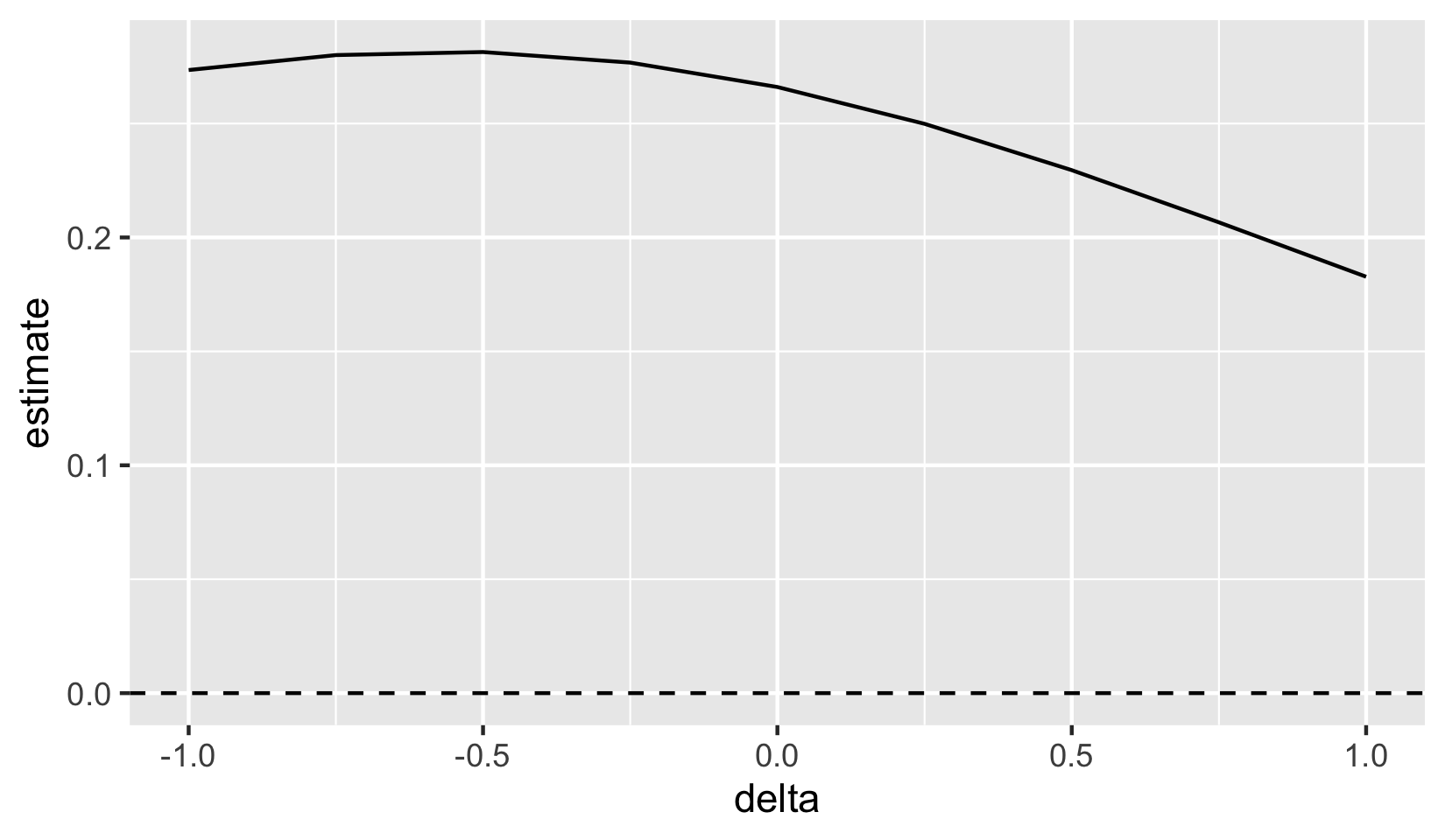
The coefficient moves smoothly with \(\delta\), so the question is whether it crosses zero inside a range of \(\delta\) you consider plausible. If it does not, the conclusion is robust to this departure from MAR; if it does, the crossing point is what the report should quote, alongside an argument about which values of \(\delta\) are credible.
mice approach.mice package documentation at amices.org/mice, package-level reference.